Hello and welcome to my complete video course about Multivariable Calculus consisting of 31 videos. This series covers all the key concepts you need to understand, presented in a logical order. Along with the videos, you’ll find helpful text explanations. You can test your knowledge using the quizzes. Additionally, PDF versions of the lessons are available for your reference. If you have any questions, feel free to ask in the community forum. Let’s get started!
Part 1 - Introduction
Multivariable Calculus is a video series I started for everyone who is interested in learning how to deal with partial derivatives, directional derivatives, and total derivatives. We discuss some important theorems like Taylor’s theorem and the Implicit Function Theorem. However, let us start with a quick overview:

Content of the video:
00:00 Intro
00:39 Prerequisites
02:15 Applications of the course
02:58 Content of the course
04:20 Credits
With this you now know the topics that we will discuss in this series. Some important bullet points are partial derivatives, directional derivatives, total derivatives and Lagrange multipliers. In order to describe these things, we need to generalise a lot from one variable to several variables. Now, in the next video let us discuss continuity.
Part 2 - Continuity
In the next part, we will extend the definition of continuity to functions of the form $ f: \mathbb{R}^n \rightarrow \mathbb{R}^m $. For this we will need a notion of distance in these higher-dimensional spaces. Therefore, we will define the so-called Euclidean distance.

Content of the video:
0:00 Intro
0:25 Continuous Functions
1:45 Continuity via sequences
2:39 Measuring distance in ℝⁿ
5:31 Convergent sequences in ℝⁿ
8:20 (Non-trivial) Link between single-variable convergence definition vs. new definition
10:33 Multivariable continuity
Part 3 - Examples of Continuous Functions
In the next part, we will look at some examples. Mostly, we show that continuity can fail at a point even if some sequences suggest continuity there. Click at the button to find the codes we used in Python to plot the 3D graphs.

Part 4 - Partial Derivatives
Now, we are finally ready to talk about derivatives in several variables. We start with the notion of partial derivatives.

Part 5 - Total Derivative
In the next video, we generalise the notion of a linear approximation as we know it for functions $ f: \mathbb{R} \rightarrow \mathbb{R} $ to multivariable functions $ f: \mathbb{R}^n \rightarrow \mathbb{R}^m $. This leads to the notion of the total derivative.

Part 6 - Partially vs. Totally Differentiable Functions
Next, we look at the difference between the terms partially differentiable and totally differentiable.

Part 7 - Chain, Sum and Factor rule
A lot of calculation rules from the one-dimensional case can be translated to this multivariable setting. In fact, the sum rule and the factor rule look exactly the same. However, the chain rule has to be modified a little but it stays one of the most important rules in calculations. For more details of the proof, please check the PDF version.

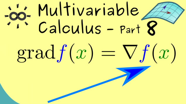
Part 8 - Gradient
In the next video, we will introduce the so-called gradient for functions $ f: \mathbb{R}^n \rightarrow \mathbb{R} $.
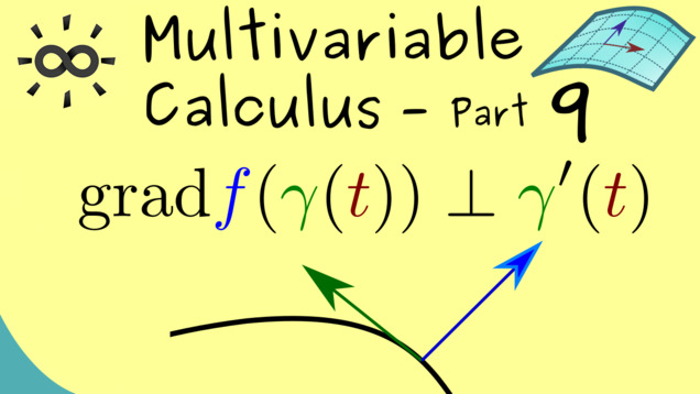
Part 9 - Geometric Picture for the Gradient
Let’s continue the discussion from the last video by visualising the gradient for functions in $ \mathbb{R}^2 $. This is a geometric view for the gradient which can be very helpful.
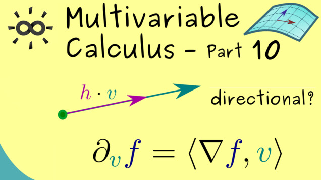
Part 10 - Directional Derivative
Now, we extend our inventory of different derivatives. We define the directional derivative for functions $ f: \mathbb{R}^n \rightarrow \mathbb{R} $ and vectors $ \mathbf{v} \in \mathbb{R}^n$.
Part 11 - Gradient is Fastest Increase
You will also hear that the gradient gives the direction of the fastest increase. In the following video, we will prove this important fact.

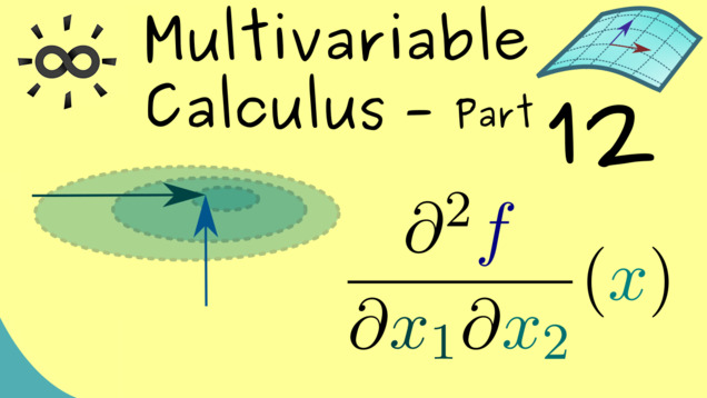
Part 12 - Second Order Partial Derivatives
In the next video, we finally introduce higher-order partial derivatives.
Part 13 - Schwarz’s Theorem
After defining the second-order derivatives, we now can show that the order for calculating the partial derivatives does not matter under some mild assumptions. This is also known as Schwarz’s Theorem, named after the German mathematician Hermann Amandus Schwarz.

Part 14 - Vector Fields and Potential Functions
As an application of Schwarz’s theorem, we can look at so-called potential functions for vector field. It turns out that there is a necessary condition for the existence of such functions.

Part 15 - Multi-Index Notation
For later and for a lot of formulas, we will need a more compact notation for partial derivatives. A very useful possibility is the so-called multi-index notation. There one just uses tupels of integers and some convenient interpretations of symbols concerning multi-indices.

Part 16 - Taylor’s Theorem
As a generalisation of the one-dimensional case, we can form polynomial approximations of differentiable functions. This is known as Taylor’s theorem.

Part 17 - Taylor’s Theorem - Examples
Now, we can also look at some examples for Taylor polynomials. We also discuss the second-order Taylor polynomial in more detail. In order to do this, we will introduce the so-called Hessian matrix, which includes the second-order partial derivatives.

Part 18 - Local Extrema
Similarly to the definition of local extrema for functions $ f : \mathbb{R} \rightarrow \mathbb{R} $, we can define them for functions $ f : \mathbb{R}^n \rightarrow \mathbb{R} $ as well. It turns out that necessary and sufficient conditions also look the same. We just have to find the correct substitutions and translations to do it.

Content of the video:
00:00 Introduction
00:42 Explaining local extrema
01:51 Definition: Local maximum and local minimum
03:10 Correction: Isolated and strict local maxima should be distinguished, see PDF!
04:12 Definition: Local extremum
04:44 Necessary condition for local extremum
06:12 Sufficient condition for local extremum
08:31 Positive definite Hessian
09:30 Negative definite Hessian
09:54 Indefinite definite Hessian
11:13 Implication from having a local extremum
12:59 Outro
Important note: I noticed that the definition of isolated local minimum that I gave in the video is not the standard one. It would be better to call it a strict local minimum instead and see the isolated local minimum as a special case of that. I corrected that in the PDF version. It does not change any of the results later.
Part 19 - Examples for Local Extrema
Let’s make everything more concrete and look at some particular examples.

Part 20 - Sylvester’s Criterion
If you know some linear algebra, the Sylvester Criterion is the way to go to check for local extrema.

Content of the video:
00:00 Intro
00:54 Assumptions of Sylvester’s Criterion
02:07 Sylvester’s Criterion for positive definite matrices
03:57 Sylvester’s Criterion for negative definite matrices
04:45 Proof for diagonal matrices
06:34 Example calculation
08:57 Credits
Part 21 - Diffeomorphisms
Let’s start with a new topic here. Recall that we want to go into the direction of the implicit function theorem. For this, we first need to know what a so-called diffeomorphism is. Roughly speaking, it is an invertible map that is continuously differentiable in both directions. We will look at some examples and counterexamples here.

Part 22 - Local Diffeomorphisms
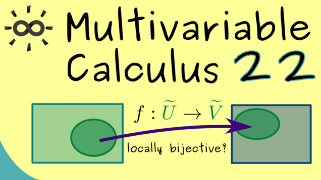
Often we have $C^1$-functions that are not even bijective so they cannot from diffeomorphisms. A good example are the polar coordinates $(r,\varphi) \mapsto \mathbb{R}^2$, where we have a $2\pi$-periodicity in the angle variable $ \varphi $. However, what we still need is a local bijectivity to use it as an alternative coordinate system. Hence, we need to introduce a new term: local diffeomorphisms.
Part 23 - Inverse Function Theorem
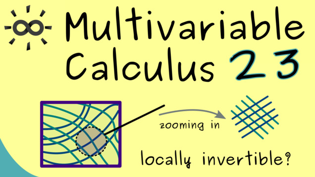
The following will be one of the main results in this course about Multivariable Calculus: the inverse function theorem. It tells us that a $C^1$-function with invertible Jacobian is already a local diffeomorphism. The proof will take some time but it has three core ideas:
- Reduce the problem to a normalized one.
- Define new functions where one can apply the Banach fixed-point theorem.
- Showing first continuity and then differentiability of the local inverse function.
Part 24 - Application of the Inverse Function Theorem
Let’s see how we can use the inverse function theorem to solve some complicated equations with several variable. This is already an appetizer for the next video where we will generalize this application.

Part 25 - Implicit Function Theorem
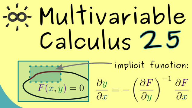
Here we see one of the main results of this course: the implicit function theorem. It generalizes the concept from the last video which showed us that an equation with several variables could be solved with respect to one variable. More precisely, we find a function, at least locally, such that the equation is represented by a graph of a function. We will formulate the theorem for general $ C^1 $-maps $ F: \mathbb{R}^k \times \mathbb{R}^n \rightarrow \mathbb{R}^n $.
Part 26 - Proof of the Implicit Function Theorem
Let’s do another proof of an important theorem! This time it’s not so complicated because we can already use the inverse function theorem here. The idea is to define a function that flattens the contour line $F(x,y) = 0$ such that we can represent it by a graph of a function. If we can also show that everything works in the $C^1$-sense, the implicit function theorem is proven.

Part 27 - Application of the Implicit Function Theorem
The implicit function theorem is very useful tool and it is used in a lot of parts of mathematics. Here we present an applications for the zeros of polynomials where the degree is to high to have a solution formula. We can still conclude that the solution is given by a $ C^\infty $-function.

Content of the video:
00:00 Introduction
00:00 Inverse Function Theorem
01:52 Implicit Function Theorem
01:52 Implicit Function Theorem
02:07 Correction: there is no connection between the two differently coloured $k$s. It would have been better to use two different symbols there.
02:56 Application of the Implicit Function Theorem for polynomials
06:09 General case of an arbitrary polynomial
09:55 Outro
Part 28 - Extreme Values With Constraints
Now we a ready to start talking about Lagrange multipliers. They stand for a whole method for solving optimization problems. This means that we want to find extrem values of a function on a given domain, which is not an open domain in $\mathbb{R}^n$ anymore. The common name for this is extrema under constraints. It turns out that it’s really easy to visualize this procedure in two dimensions.

Part 29 - Method of Lagrange Multipliers
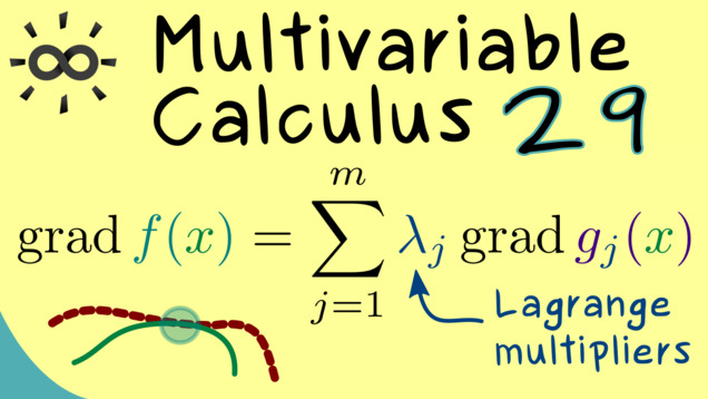
Let’s formulate the necessary condition for extrema of a function under constraints, called the method of Lagrange multipliers. We will also discuss the ideas you need for the proof and explicitely write them down for the two-dimensional case.
Part 30 - Example for Lagrange Multipliers
After all these theoretical explanations, we can apply them to a concrete example. Let’s search for extrema of a function $f: \mathbb{R}^3 \rightarrow \mathbb{R}$ under two contraints. However, don’t forget that the Lagrange multipliers only give a necessary condition. To find sufficient conditions for the candidates we get, we have to use some more knowledge about the given function.
Part 31 - Lagrangian
The method of Lagrange multipliers is a good tool for finding extrema of a given function subject to contraints. However, it might be hard to remember because it looks so different compared to the standard way of finding extrema (without constraints). A good possibility to align these procedures is to introduce the so-called Lagrangian function $ L: \mathbb{R}^n \times \mathbb{R}^m \rightarrow \mathbb{R} $ and ask about the points where the gradient of $ L $ vanishes.

This ends the series about Multivariable calculus but not the discussion about functions in $\mathbb{R}^n$. There is still a lot to say, for example, how to integrate functions over a high-dimensional domain. Let’s do that in the series Integration in Higher Dimensions.
Connections to other courses
Summary of the course Multivariable Calculus
-
You can download the whole PDF here and the whole dark PDF.
-
You can download the whole printable PDF here.
-
Test your knowledge in a full quiz.
- Ask your questions in the community forum about Multivariable Calculus.
Ad-free version available:
Click to watch the series on Vimeo.