Hello and welcome to my complete video course about Abstract Linear Algebra consisting of 52 videos. As a supporter of the channel, you can also download my book. This series builds on the original Linear Algebra course, diving deeper into more abstract concepts, like the Spectral Theorem and important matrix decomposition. Alongside the videos, you’ll find additional text explanations to help reinforce the material. To test your knowledge, use the quizzes, and refer to the PDF versions of the lessons whenever needed. If you have any questions, feel free to participate in the community discussion forum. Without further ado, let’s get started!
Part 1 - Vector Space
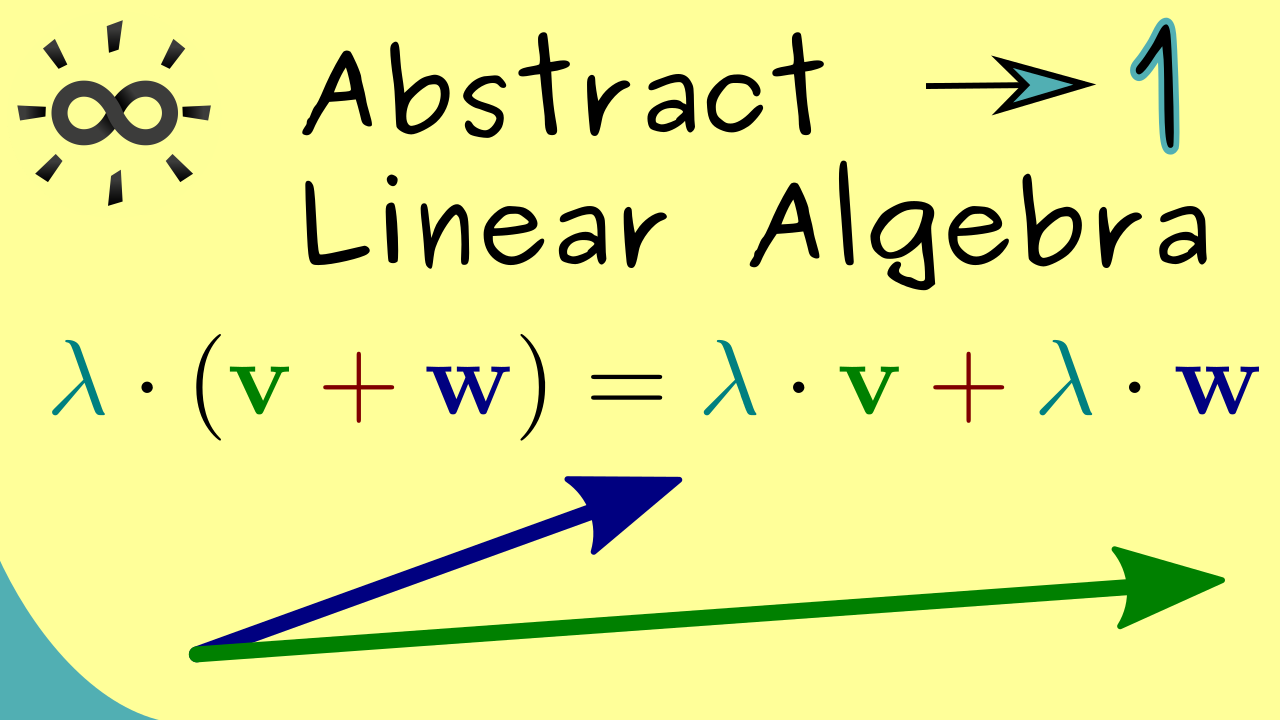
Let’s start the series by defining a general vector space. From now on, we will always remember that we need 8 rules to check if something is a vector space.
Content of the video:
00:00 Introduction
00:28 Prerequisites
01:28 Overview
03:40 Definition of a vector space
05:56 Operations on vector spaces
08:10 8 Rules on these operations
Part 2 - Examples of Abstract Vector Spaces
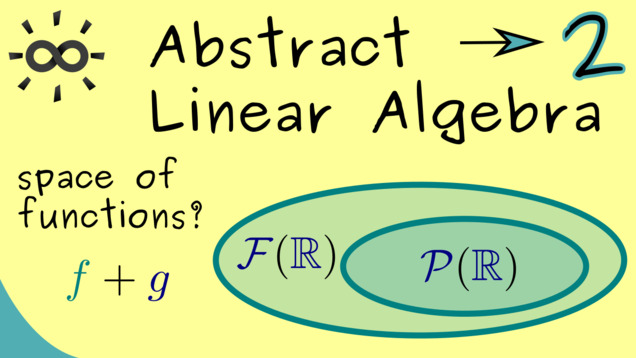
In this video, we will look back at the set of matrices and show again that they form a vector space. In addition, we will also look at more abstract examples, like function spaces and polynomial spaces. There we will already see that a lot of notions from the Linear Algebra course can be reused.
Content of the video:
00:00 Introduction
00:36 Definition of a vector space
01:39 Examples
02:48 Function Spaces
08:01 Polynomial Space
10:00 Linear Subspace
11:55 Credits
Part 3 - Linear Subspaces
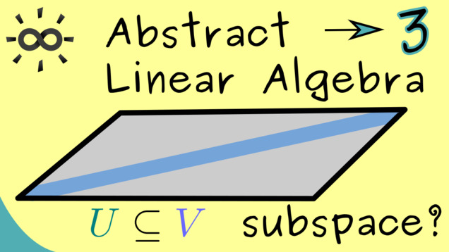
In this third part, we are finally ready to generalize the notion of subspaces. We will see that the polynomial space is a subspace contained in the general function space.
Content of the video:
00:00 Introduction
00:36 Abstract vector space
01:38 Behaviour of the zero vector
03:00 Proof for the formulas
07:13 Linear subspaces = special vector spaces
10:00 Definition of linear subspace
12:02 Example quadratic polynomials
14:07 Credits
Part 4 - Basis, Linear Independence, Generating Sets
Now we are ready to generalize the notion of a basis for abstract vector spaces. Essentially, the definitions look exactly the same as for $ \mathbb{R}^n $ and $ \mathbb{C}^n $. However, it’s good to formulate them again and point out the small differences in this generalization.

Content of the video:
00:00 Introduction
00:36 Definition of polynomial spaces
02:27 Definition: linear combination
03:38 Definition: span of a subspace
04:44 Definition: generating set for a subspace
05:29 Definition: linear independent sets
06:36 Definition: basis of a subspace
07:57 Definition: dimension of a subspace
09:18 Examples for polynomial spaces
11:25 Example for infinite-dimensional vector space
11:44 Example for matrices
12:42 Credits
Part 5 - Coordinates and Basis Isomorphism
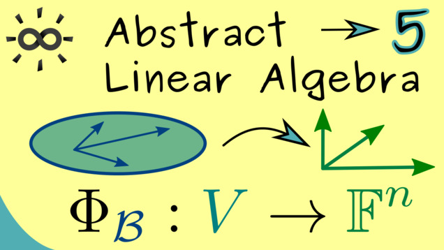
After fixing a basis in an abstract vector space, one can use that to translate this space to the very concrete space $ \mathbb{F}^n $. This translation is called the basis isomorphism, written as $ \ \Phi_{\mathcal{B}} $.
Content of the video:
00:00 Introduction
00:37 Assumptions
02:31 Definition: Coordinates with respect to a basis
03:40 Coordinate vector
03:58 Picture for the idea
06:44 Definition: basis isomorphism
08:32 Credits
Part 6 - Example of Basis Isomorphism
This video explains the basis isomorphism with some examples. We see that it is a very natural construct that helps to analyze abstract vector spaces, as long as they are finite-dimensional. In particular, we show how we can prove that vectors from a function space like $ \mathcal{P}(\mathbb{R}) $ are linearly independent.

Content of the video:
00:00 Introduction
00:33 Span in the function space
01:27 Is this a basis?
02:03 Checking for linear independence
05:40 Reformulating as matrix-vector multiplication
06:52 Uniquely solvable?
08:52 Basis isomorphism
11:16 Credits
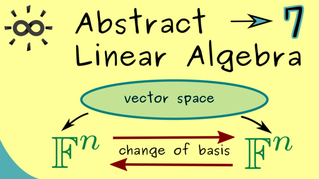
Part 7 - Change of Basis
The next videos will cover the subject of changing a basis in a vector space. This means that we have to combine twwo basis isomorphisms. This change of basis is very important because often we want to choose a suitable basis for solving a given problem. Hence, we need to know how switch bases in an effective way.
Content of the video:
00:00 Introduction
00:44 Two bases for a vector space
02:53 Change of basis
03:20 Basis isomorphism properties
04:13 Example (change of basis in polynomial space)
07:35 Switching from old to new coordinates
09:35 Change of basis is a linear map
10:57 Credits
Part 8 - Transformation Matrix
Now we can put the change-of-basis map in the form of a matrix. This change-of-basis matrix has some different names, like transformation matrix or transition matrix. However, it simply describes what happens to the basis vectors like what we learnt in the original Linear Algebra course.

Content of the video:
00:00 Introduction
00:47 Picture for change of basis
02:01 What happens with the first unit vector?
03:23 Representation by a matrix
04:24 Change-of-basis matrix
05:20 Picture for the transition matrix
06:40 Inverse of the transformation Matrix
07:10 Example with polynomials
10:38 Credits
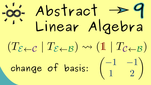
Part 9 - Example for Change of Basis
After all this theoretical talk, we finally want to look at concrete example. Indeed, we can take the vector space $ \mathbb{R}^2 $ and do a change of basis there. It turns out that this is a general calculation scheme one can also use in higher dimensions.
Content of the video:
00:00 Introduction
00:39 Change-of-basis matrix
01:58 Example - explanation
02:50 Example in R²
05:10 First transition matrix
05:54 Second transition matrix
06:39 Composition of change-of-basis
07:51 Gaussian elimination for product
11:41 Credits
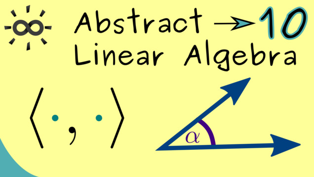
Part 10 - Inner Products
Let’s go to an easier topic again. We already know from the Linear Algebra course that measuring lengths and angles can be generalized. Now, we can also describe inner products for more abstract vector spaces, like the polynomial space.
Content of the video:
00:00 Introduction
00:37 Extension of notations
02:13 Definition: inner product
02:52 Positive definite
04:23 Linear in the second argument
05:50 Conjugate symmetric
06:50 Standard inner product
08:10 Non-standard inner product
09:37 Integral inner product on polynomial space
13:26 Credits
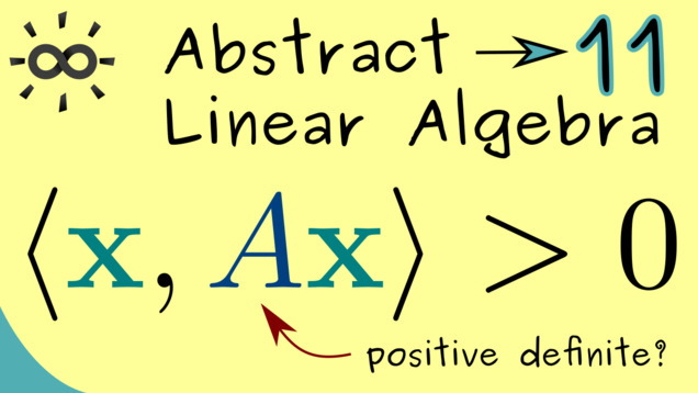
Part 11 - Positive Definite Matrices
This is very concrete topic about matrices. However, since positive matrices play a crucial role for defining inner product, we discuss them now in more detail.
Content of the video:
00:00 Introduction
00:45 Example: inner product in F²
02:30 Checking rules for inner product
03:20 Definition: positive definite matrix
04:30 Positive definite matrices define inner products
05:24 Example revisited
07:21 Example of a positive definite matrix
07:56 Equivalent statements for positive definite matrices
09:48 Sylvester’s criterion
12:14 Example for Sylvester’s criterion
13:07 Example for Gaussian elimination
14:38 Credits
Part 12 - Cauchy-Schwarz Inequality
You can remember that inner product are used to give a geometry to the the vector space. This means that it is possible to measure angles between vectors and lengths of vectors. In particular $ | x | = \sqrt{\langle x, x \rangle} $ defines a so-called norm. The relation to the inner product and this iduced norm is stated in the famous Cauchy-Schwarz inequality, which will prove now:

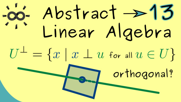
Part 13 - Orthogonality
After discussing general inner products, we know that they can describe geometry in general vector spaces. In particular, the notion of orthogonal vectors make sense. So even in abstract vector spaces, we can say that the vector $ x $ is perpendicular to $ y $ and we write it as $ x \perp y$.
Part 14 - Orthogonal Projection Onto Line
Here we start with an important topic: orthogonal projections. It’s a very visual concept if you imagine an object that produces a shadow because the sun is above it. Indeed, this gives exactly the correct picture if you represent a vector by an arrow and introduce a right-angle for this projection. The nice thing is that this visualization also works in our abstract vector spaces. Let’s start this disussion in a one-dimensional case.

Part 15 - Orthogonal Projection Onto Subspace
We already know the orthogonal projection onto a one-dimensional line. Now, we should be able to generalize this to a finite-dimensional subspace of our vector space. Indeed, the visualization looks very similar because we still search for a decomposition $ \mathbb{x} = \mathbb{p} + \mathbb{n} $ where $ \mathbb{p} $ lies in the subspace and $ \mathbb{n} $ is orthogonal to it.

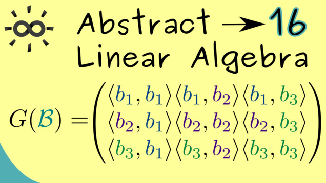
Part 16 - Gramian Matrix
To calculate the orthogonal projection from the last part, we need to solve a system of linear equations. This one can be represented by the so-called Gramian matrix.
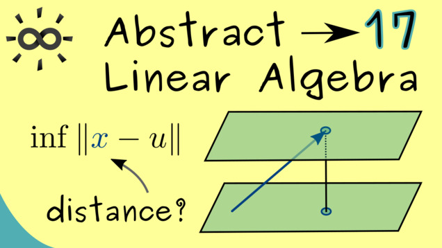
Part 17 - Approximation Formula
After all the calculations for orthogonal projections, we can give another motivation why these projections are so important, especially in the abstract settings. The approximation formula shows that the orthogonal projection minimizes the distance between the point and the subspace, a property that can be useful whenever such a minimizer is needed.
Part 18 - Orthonormal Basis
For calculating the orthogonal projection, we had to solve a system of linear equations given by the Gramian matrix. The system would be already completely solved if the matrix is in diagonal form.This leads to the notion of an orthogonal basis and of an orthonormal basis, usually abbreviated by (ONB).

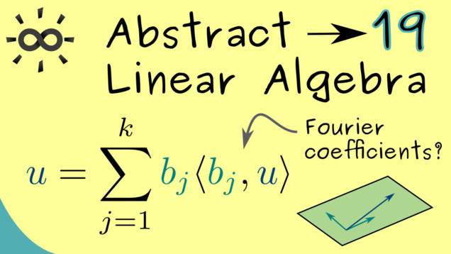
Part 19 - Fourier Coefficients
The name Fourier expansion and Fourier coefficients are often used in a special context, discussed in the video series Fourier Transform. However, they also make sense in the abstract description of an ONB in a general vector space.
Part 20 - Gram-Schmidt Orthonormalization
In the following, we will explain how we take any basis in a finite-dimensional vector space with inner product and transform it into an orthonormal basis. This is known as the Gram-Schmidt process. It is useful when you need an ONB to make your calculations simpler. We will seed that the algorithm is not complicated at all since it essentially just uses the orthogonal projections we already know.

Part 21 - Example for Gram-Schmidt Process
After just explaining the algorithm in the last video, we can put some life to it. It’s a good exercise to do some orthonormalization in the vector space $ \mathbb{R}^n $ to see the algorithm in work. However, here we present a more abstract example: we will consider polynomials. In fact, these procedure will lead to the so-called Legendre polynomials.

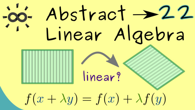
Part 22 - Linear Maps
Here, we will discuss linear maps as we have done it for maps between $ \mathbb{R}^n $ and $ \mathbb{R}^m $ already. However, now we do it in the general setting for arbitrary general vector spaces. The definition looks the same since a linear map has to conserve the linear structure of the vector space.
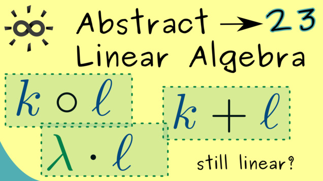
Part 23 - Combinations of Linear Maps
A linear map conserves the linear structure of the vector space. It turns out that this is still the case if we combine linear maps in some special way. We discuss the addition and the composition of linear maps.
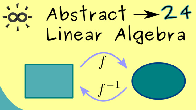
Part 24 - Homomorphisms and Isomorphisms
Let’s quickly talk about inverses of linear maps. As for the special linear maps $ f: \mathbb{R}^n \rightarrow \mathbb{R}^m $, it turns out that inverses of linear maps are also linear. Usually one speaks of isomorphims in this case.
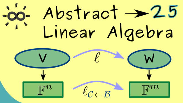
Part 25 - Matrix Representation for Linear Maps
A linear map between finite-dimensional vector spaces can completely be described by an ordinary matrix. One only has to fix two bases in domain and codomain.
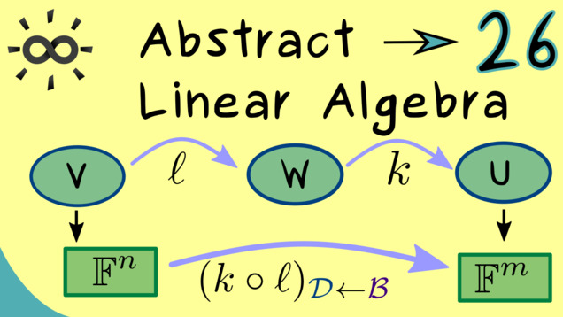
Part 26 - Matrix Representations for Compositions
Matrix representations can help a lot if you want to combine some linear maps. In this case, one can just use the matrix product of the corresponding matrix representation if one chooses the same basis for the vector space in the middle. Let’s see how this looks in detail:
Part 27 - Change of Basis for Linear Maps
We have already learnt how to use the change-of-basis matrix to switch between different bases on a vector space. Now we can also use this to see the connection between two different matrix representations for a linear map $ \ell: V \rightarrow W $.

Part 28 - Equivalent Matrices
With the example from the last video, we have seen two matrices that represent the same linear map, just with respect to different bases of the corresponding vector spaces. Now, a natural question could be how to decide if two given matrices can represent the same linear map. Obviously, there has to be some criterion for two matrices because the zero matrix only represents the zero linear map and there is no other matrix which does that. The connection we are searching is usually summarized as equivalent matrices.
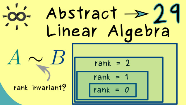
Part 29 - Rank gives Equivalence
We quickly find that equivalent matrices can be described by considering their ranges and kernels. However, only the dimensions do not change under the equivalence transformation. This, together with the rank-nullity-theorem, leads us to the fact that the equivalence classes for the space of matrices are completely given by the rank.
Part 30 - Similar Matrices
We can also look at linear maps $\ell: V \rightarrow V$, so the maps that send a vector space to itself. Obviously, these linear maps have square matrices as their matrix representations and one can even choose matrix representations with respect to a single basis $\mathcal{B}$, written as $\ell_{\mathcal{B} \rightarrow \mathcal{B}}$. Hence, a natural question is how these matrices are related to each other and this lead to the concept of similarity.
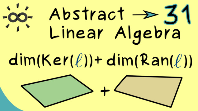
Part 31 - Solutions for Linear Equations
Of course, a general linear map can also describe a linear equation where we can ask for the solution set. It turns out that, by using matrix representation, we already know everything about this solution set. However, it is still a good idea to formulate it in this general case as well. For that we have to define the notions range and kernel for linear maps. Moreover, we also get the rank-nullity theorem for general linear maps between finite-dimensional vector spaces.
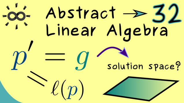
Part 32 - Example for General Linear Equation
Let’s discuss a example for solving general linear systems. As often the polynomial space can be used as a convenient one.
Part 33 - Extension of Determinant
By using matrix representations, we can also extend the notion of the determinant, which is a volume function in Linear Algebra. It’s an advantage to have this also for abstract linear maps.

Part 34 - Eigenvalues and Eigenvectors for Linear Maps
The notion of eigenvalues and eigenvectors also works for linear maps as we have already discussed it before in the Linear Algebra course.. Moreover, the definition does not require a finite-dimensional vector space such that we can formulate it in a really general way. However, for explicit calculations we would definitely prefer a finite-dimensional vector space such that we can use a matrix representation. Everything beyond that is actually discussed in the Functional Analysis course. We can look at example to get a glimpse why eigenvectors are still useful there.

Part 35 - Definition of Jordan Normal Form
Let’s start talking about the theory behind the Jordan normal form. We will show that each square matrix with complex numbers as entries is similar to a triangular matrix. In particular, this triangular matrix can be chosen as a Jordan normal form, which will define in this video. If you want to see more examples, you can check out the other series I have about the Jordan normal form.

Part 36 - Generalized Eigenspaces
We already know that the Jordan normal form is only needed for non-diagonalizable matrices because otherwise we can just use a diagonal matrix instead. However, for such a matrix there is an eigenvalue where the dimension of the corresponging eigenspace is smaller than the algebraic multiplicity. Hence, we don’t have enough eigenvector directions to get a diagonalization. Now the question is: how to substitute these missing directions? That where the so-called generalized eigenvectors come in. These are not eigenvectors but they become eigenvectors when we multiply them by $(A - \lambda \mathbf{1})^{k-1}$ for a suitable natural number $k$. We speak of generalized eigenvectors of rank $k$ in that case. Let’s discuss the details!

Part 37 - Fitting Index
The Fitting index is named after a German mathematician called Fitting but it turns out that the name is quite fitting because the index tells us which generalized eigenspace fits in as the largest possible one. This result we can use to define the transformation to the Jordan normal form in the end.

Part 38 - Invariant Subspaces
For our journey to the Jordan normal form, we will also need the important concept of invariant subspaces. These are easy to characterize: if we can restrict the linear map to a subspace where the codomain is also this subspace, then we say the subspace in invariant under the linear map.

Part 39 - Direct Sum of Subspaces
It might not surprise you that you can combine two subspaces and get a new subspace out that contains both of them. The procedure is quite simple: just form the union of both subspaces and take the span of it. However, the direct sum of subspaces puts an additional requirement in. Namely, the subspaces should only have a trivial intersection. Let’s do that in more detail and explain why we need this for the Jordan normal form proof.

Part 40 - Block Diagonalization
We already learnt about block matrices as a special representation of matrices. Especially for the calculation of determinants, such a block form was helpful. Now we will show under which conditions, we can bring a given matrix into a block diagonal form.

Part 41 - Algebraic Multiplicity with Fitting Index
Now we can use the result from the last video to connect the block diagonalization to the eigenvalues of the matrix. It turns out the algebraic multiplicity is actually given by the dimension of the largest generalized eigenspace. There we already know that this one is described by the Fitting index.

Part 42 - Jordan Chains
Combining everything from the last videos results in the Jordan normal form. In order to explain the explicit form of the Jordan boxes, we have to construct suitable generalized eigenvectors. This is done by so-called Jordan chains. Please note that some technical details about this construction are added in the PDF version.

Part 43 - Example for Jordan Normal Form
After all these discussions about the theory of the Jordan normal form, we can finally look at an example calculation. We will see how we can actually form the Jordan chains for a given square matrix. If you want to see more example calculations, you can watch my separate short videos series about it.

Other videos related to this topic:
- Jordan Normal Form 1 | Overview
- Jordan Normal Form 2 | An Example
- Jordan Normal Form 3 | Another Example
- Jordan Normal Form 4 | Transformation Matrix
Part 44 - Application for Jordan Normal Form
To finish our long discussion about the Jordan normal form, I want to show you some really common applications. First, it can be used to get some general formulas for the determinant and the trace of a square matrix (where the trace is sum of the diagonal). In particular, the determinant is always given by the product of eigenvalues and the trace is the sum of the eigenvalues. Second, the matrix exponential, defined as a power series of matrices, can be calculated by using the transformation into the Jordan normal form.

Other videos related to this topic:
Part 45 - Schur Decomposition
The Schur decomposition transforms any complex matrix into a Schur normal form, which is an upper triangular matrix. So it sounds like the Jordan normal form but it’s different since the similarity transformation should be done with unitary matrices. Note that the inverse of a unitary matrix is easy to calculate and this is the big advantage of this decomposition procedure.

Part 46 - Example of Schur Decomposition
We have presented the whole algorithm in the last video. Now we can use it and show an explicit calculation for a $3 \times 3$ matrix.

Part 47 - Spectral Theorem for Normal Matrices
Let’s look at a special case of the Schur decomposition. Namely, the one where the upper triangular matrix is actually a diagonal matrix. This is what we would call unitarily diagonalizable. It turns out that these matrices are exactly the normal matrices. It’s a very important result in Linear Algebra and known as the spectral theorem.

Part 48 - Proof of Spectral Theorem
Now we are ready to formulate the proof of the spectral theorem for normal matrices. We will need the Schur decomposition.

Content of the video:
00:00 Introduction
00:40 Statement: Spectral Theorem for Normal Matrices
01:37 Proof of first implication
04:15 Proof of second implication
06:15 How do normal triangular matrices look like?
08:31 Induction proof that normal triangular matrices are diagonal
12:06 Correction: here we already use $w = 0$ for the matrix product of $R^{\ast}R$!
12:27 Using the induction hypothesis
13:45 Outro and credits
Part 49 - Singular Value Decomposition (Overview)
The next matrix decomposition is one of the most important ones, simply because it’s very general and used a lot in applications. It even works for rectangular matrices and we call it the singular value decomposition. Let’s first give an overview what we want there before we explain the name.

Part 50 - Singular Values and Singular Vectors
In order to calculate the singular value decomposition (SVD), we have to know what singular values and singular vectors actually are. Indeed, they are completely related to eigenvalues and eigenvectors, which also means that we have to talk about square matrices. More concretely, we consider the self-adjoint matrices $ A^\ast A $ and $ A A^\ast $.

Part 51 - Singular Value Decomposition (Algorithm and Example)
After we already discussed the definition of singular values and how the SVD has to look like, we can finally write down the whole construction procedure. This algorithm is something you would apply in your pen-and-paper calculation. We also demonstrate it with an explicit example for a $2 \times 2$ matrix.

Part 52 - Singular Value Decomposition (Application)
It turns out that the SVD can be used for a low-rank approximation for matrices. For this only the singular values with the largest contribution are considered. Let’s discuss how we can define such a matrix of lower rank and let’s apply it to an compression method of photos.

This was the last video in the course but not the last video where we talk about eigenvalues, the spectral theorem, and self-adjoint operators. You should definitely check the video series about Functional Analysis and Hilbert spaces!
Connections to other courses
Summary of the course Abstract Linear Algebra
-
You can download the whole PDF here and the whole dark PDF.
-
You can download the whole printable PDF here.
-
Test your knowledge in a full quiz.
- Ask your questions in the community forum about Abstract Linear Algebra.
Ad-free version available:
Click to watch the series on Vimeo.