Here, you find my whole video series about Probability Theory in the correct order and I also help you with some text around the videos. If you want to test your knowledge, please use the quizzes, and consult the PDF version of the video if needed. When you have any questions, you can use the comments below and ask anything. However, without further ado let’s start:
Part 1 - Introduction (including R)
Probability Theory is a video series I started for everyone who is interested in stochastic problems and statistics. We can use a lot of results that one can learn in measure theory series. However, here we will be able to apply the theorems to probability problems and random experiments. In order to this, we will use RStudio along the way:

Content of the video:
00:00 Introduction
01:20 simple example: throwing a die
02:54 Rstudio
05:17 Outro
With this you now know the topics that we will discuss in this series. Some important bullet points are probability measures, random variables, central limit theorem and statistical tests. In order to describe these things, we need a good understanding of measures first. They form the foundation of this probability theory course but we do not need to go into details. Now, in the next video let us discuss probability measures.
Part 2 - Probability Measures
The notion of a probability measure is needed to describe stochastic problems:

Content of the video:
00:00 Idea of a probability measure
01:40 Requirements
04:19 Sigma algebra
05:50 Sigma additivity
06:31 Definition probability measure
07:22 Example
08:57 Exercise about properties of probability measures
09:30 Outro
Part 3 - Discrete vs. Continuous Case
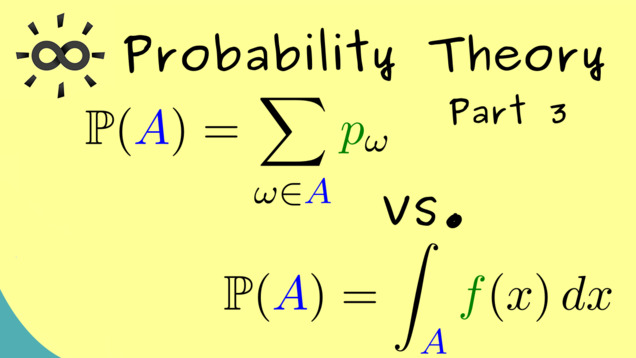
We distinguish discrete and continuous cases because they often occur in applications. Note that for the discrete case, we have a so-called probability mass function, and for the continuous case, we have a so-called probability density function.
Content of the video:
00:00 Intro
00:48 Introduction of cases
02:17 Sample Space (discrete case)
02:33 Sample Space (continuous case)
03:14 Sigma algebra (discrete case)
03:36 Sigma algebra (continuous case)
03:59 Probability measure (discrete case)
05:41 Probability measure (continuous case)
07:46 Example (discrete case)
08:44 Example (continuous case)
10:38 Outro
10:57 Endcard
Part 4 - Binomial Distribution
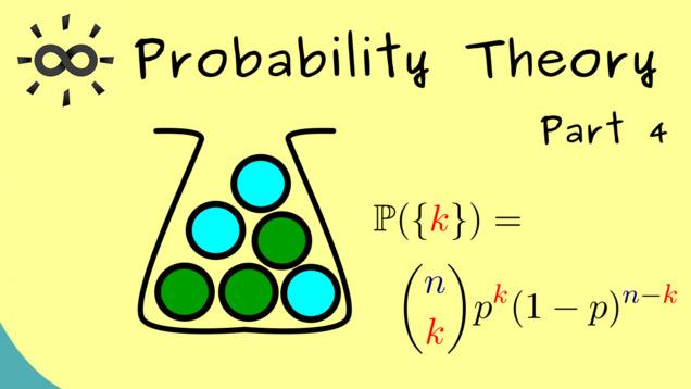
Now we talk about a special discrete model: the binomial distribution. It occurs when we toss a coin n times and count the heads. Alternatively, we could draw n balls, with replacement, from a urn with two different kinds of balls:
Content of the video:
00:00 Intro
00:10 Binomial distribution
06:27 Binomial distribution in RStudio
09:40 Urn model in RStudio
14:55 Comparison of urn model and rbinom in RStudio
15:36 Endcard
Part 5 - Product Probability Spaces
Now we talk about product spaces, which will be very important for constructions of probability spaces:

Part 6 - Hypergeometric Distribution
The next discrete model we will discuss is the so-called hypergeometric distribution. It is related to the binomial distribution in an urn model. However, now we will draw without replacement.

Content of the video:
00:00 Intro
00:13 Hypergeometric distriubution
02:21 Writing a sample space for Hypergeometric function
05:42 Hypergeometric distribution for 2 colours
07:06 Hypergeometric distribution in R
10:29 Outro
Part 7 - Conditional Probability
In the next video, we start with a very important topic: conditional probability.

Content of the video:
00:00 Intro
00:26 Conditional Probability (definition)
05:12 example
09:09 Outro
Part 8 - Bayes’s Theorem and Total Probability
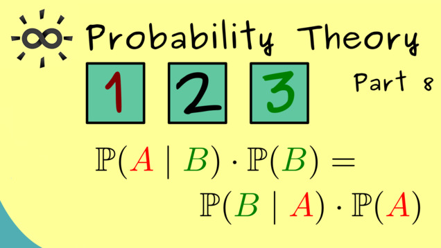
Now we are ready to discuss a famous theorem: Bayes’s theorem. We also talk about the related law of total probability and illustrate both things with the popular Monty Hall problem.
Content of the video:
00:00 Intro
00:17 Bayes’s theorem
01:20 Law of total Probability
04:51 Example: Monty Hall problem
09:35 Outro
Part 9 - Independence for Events
Next, we talk about an important concept: independence. We start by explaining the independence of events. First we just have two events but then we consider infinitely many.

Content of the video:
00:00 Intro
00:19 Visualization (Independence for events)
03:48 Definition of independence
04:52: Example (discrete case)
07:38 Continuous case
10:52 Outro
Part 10 - Random Variables
We are ready to introduce random variables. It turns out that the definition is not complicated at all. Nevertheless, we often use them to extract the important parts of a random experiment.

Content of the video:
00:00 Intro/ short introduction
00:56 Example (discrete)
02:57 Definition of a random variable
04:56 Continuation of the example
07:49 Notation
09:28 Outro
Part 11 - Distribution of a Random Variable
Next, we want to introduce the notion of distribution of a random variable. This is not a complicated concept but, in fact, it will be crucial in all upcoming videos.

Part 12 - Cumulative Distribution Function
We continue with the cumulative distribution function for a random variable. It is often just called CDF.

Part 13 - Independence for Random Variables
Now let us define the notion of independence for random variables. We will use the definition of independence for events for this:

Part 14 - Expectation and Change-of-Variables
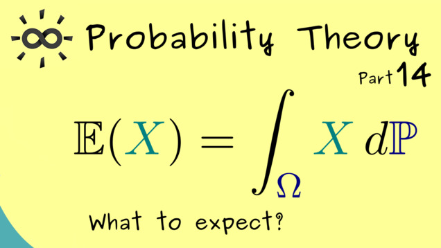
The next concept is one of the most important ones. We talk about the expectation of a random variable. You also find a lot of other names for that, for example, expected value, first moment, mean, and expectancy.
Part 15 - Properties of the Expectation
Now let’s look at some more examples and some important properties of the expectation like linearity:

Part 16 - Variance
We continue with another important concept: variance. With this we can measure how much a random variable deviates from its mean.

Part 17 - Standard Deviation
Now we expand the notion of the variance and define the so-called standard deviation. We consider some examples. Most importantly, we discuss the normal distribution and visualize it in RStudio.

Part 18 - Properties of Variance and Standard Deviation
In the next video, we prove some properties of the variance, which can be extended to properties for the standard deviation. In particular, for independent random variables, the variance is additive.

Content of the video:
00:00 Intro
00:35 Properties
01:30 Variance is additive
01:50 Scaling variance
02:20 Scaling standard deviation
03:04 Proof of properties
07:48 Credits
Part 19 - Covariance and Correlation
In this video, we will extend the variance function from the last videos to two random variables. Therefore, it will measure how correlated the random variables are.

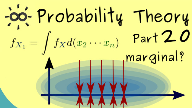
Part 20 - Marginal Distributions
In this video, we discuss how we can restrict random variables in several dimensions to ordinary random variables.
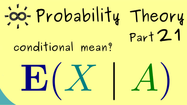
Part 21 - Conditional Expectation (given events)
In this video, we introduce a new concept for the conditional probability: the so-called conditional expectation. It explains what we expect as a outcome of a random variable under the condition described by an event. We remember the particular formula by using an indicator function, written as $ \mathbf{1}_B $.
Part 22 - Conditional Expectation (given random variables)
We extend the notion from the last video for conditions given by another random variable. This means that the, here defined, conditional expectation is a random variable.

Part 23 - Stochastic Processes
With this video, we start a new topic about stochastic processes, which are often used in applications. First, we give the definition and then we look at some simple examples.

Part 24 - Markov Chains
Most of the time, the stochastic processes we consider have some additional properties. A so-called Markov process does not need the past to calculate the future. The present state is enough for this.

Part 25 - Stationary Distributions
Let’s continue the discussion from the last video where we already introduced the transition matrix for a time-homogeneous discrete-time Markov chain. This one can help us to find so-called stationary distributions for the given Markov chain. One just have to solve an eigenvalue equation as we learnt it in Linear Algebra.

Part 26 - Markov’s Inequality and Chebyshev’s Inequality
Now, we start the journey to discuss the famous central limit theorem. In order to that, we will need some technical results first. We begin by stating and proving two popular estimates for probabilities. The first one is Markov’s inequality, which gives us a rough estimate of an integral, and the second one is Chebyshev’s inequality (also called the Bienaymé–Chebyshev inequality). It gives an upper bound for the probability of being off from the mean.

Content of the video:
00:00 Intro
00:42 General assumption
01:11 Markov’s inequality
02:42 Visualization of Markov’s inequality
04:32 Proof of Markov’s inequality
07:10 Chebyshev’s inequality
09:11 Proof of Chebyshev’s inequality
11:42 Credits
Part 27 - kσ-intervals
As an application of Chebyshev’s inequality, we try to estimate the so-called k sigma intervals. These describe the probability to find values in an interval around the mean. Here, $ \sigma $ simply stands for the standard deviation of the given random variable. We will also explain the 68–95–99.7 rule one has for the normal distribution.

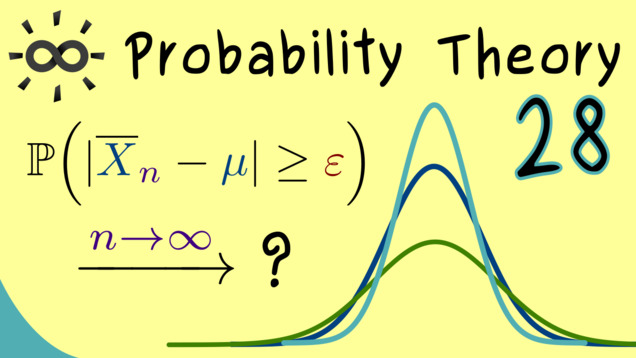
Part 28 - Weak Law of Large Numbers
In the next videos, we will talk a lot about the convergence of random variables. In particular, we will define different notions for particular types of convergence. In the first step, we see what it means that a random variable converges in probability. A special case of that is given in the weak law of large numbers, which states the empirical probability of an event $A$, given by the relative frequency of the given event, converges to the actual theoretical probability $ \mathbb{P}(A) $.
Part 29 - Monte Carlo Integration
If we speak of Monte Carlo methods, we mean some specific numerical methods to calculates some quantities in an approximate way. The idea behind it is to use the law of large numbers to estimate the quantity given as $ \mathbb{E}(X) $. If the number repitition is high, we also have a high probability that the calculated average lies close the expected value. We demonstrate this procedure for the calculation of a definite integral.

Part 30 - Strong Law of Large Numbers
It turns out that we can make the claim of the law of large numbers even stronger. Exactly with the same assumptions, we can formulate the so strong law of large numbers, which talks about the pointwise convergence of random variables rather than about the convergence of a probability like we have in it in the weak law.

Part 31 - Central Limit Theorem
The so-called central limit theorem explains why the normal distribution is found in so many different places. Roughly said, every probability distribution converges to the normal distribution if we look at the average and increase the sample size more and more. In this video, we explain this in correct mathematical terms and also state the assumptions one needs.

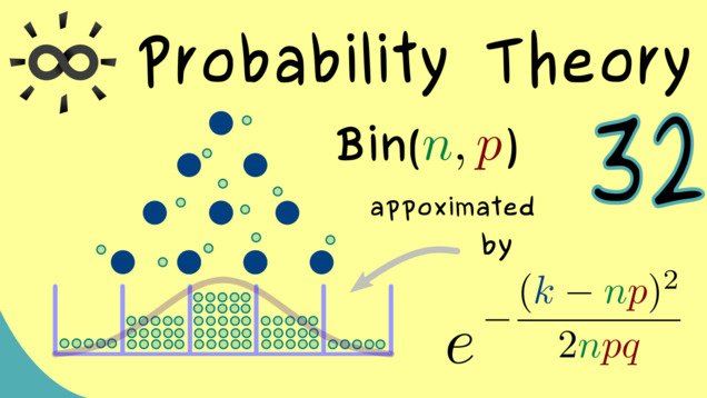
Part 32 - De Moivre–Laplace theorem
A special version of the central limit theorem can be stated for the binomial distribution. This is usually known as the De Moivre–Laplace theorem.
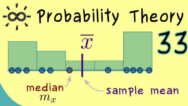
Part 33 - Descriptive Statistics (Sample, Median, Mean)
Let’s finally start talking about statistics, which will give us mathematical tools to analyze data and make predictions with them. However, before we start with the subject of inferential statistics, we will first define a lot of terms which are used a lot, like sample, median, sample mean, and sample variance. Since these terms just describe a given data set without making any predictions yet, we speak of descriptive statistics.
Summary of the course Probability Theory
- You can download the whole PDF here and the whole dark PDF.
- You can download the whole printable PDF here.
- Test your knowledge in a full quiz.
- Ask your questions in the community forum about Probability Theory
Ad-free version available:
Click to watch the series on Vimeo.