Hello and welcome to my ongoing video course about Fourier Transform, already consisting of 36 videos. The videos are arranged in the correct order to guide you through the topic step by step. Along with the videos, I offer helpful text explanations. To test your understanding, feel free to use the quizzes and refer to the PDF versions of the lessons when needed. If you have any questions, the community forum is available for discussion. Now, let’s dive right in!
Part 1 - Introduction
Let’s start by explaining what we will cover in this course. We will start with a discussion about Fourier series for periodic functions. This is an important topic to understand while the Fourier transform as an integral transform actually makes sense. After this, we can define the continuous Fourier transform and discuss the properties. Especially for the first part, we will need a lot of Linear Algebra topics, especially about inner products and orthonormal bases.

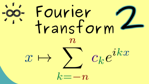
Part 2 - Trigonometric Polynomials
Let’s start with the discussion of Fourier series. For this, we first have to define what a so-called trigonometric polynomial is. We will describe the real version of these and the complex version. Both are essentially equivalent but for the introduction into the topic, the representation with sine and cosine functions is easier to visualize.
Part 3 - Orthogonal Basis
We consider the vector space $ \mathcal{P}_{2 \pi -per} $ of the real trigonometric polynomials together with an inner product. This means that the notion orthogonality makes sense. In particular, the sine and cosine functions are perpendicular. It turns out that we find an orthogonal basis for this vector space.

Content of the video:
00:00 Introduction
00:45 Real trigonometric polynomials
01:30 Subspace of trigonometric polynomials
02:41 Inner product for trigonometric polynomials
04:11 Examples
11:54 Result: OB for trigonometric polynomials
12:55 Credits
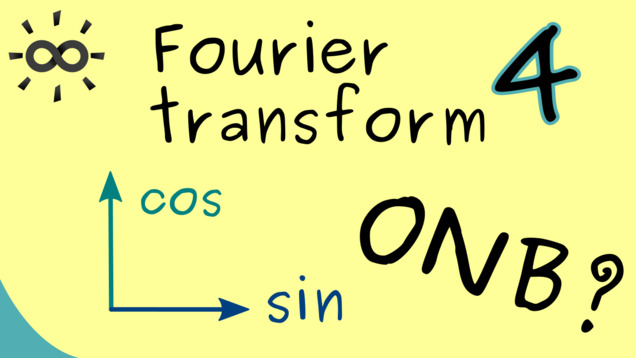
Part 4 - Orthonormalbasis of Trigonometric Functions
After finding an orthogonal basis in the last video, we can ask the question if we also have a nice orthonormal basis, where every vector is normalized with respect to the given inner product. This is possible if we scale the standard cosine and sine functions with a suitable constant. Alternatively, it’s also possible to scale the inner product to get an orthonormal basis. Here, we consider three possible cases for such an inner product.
Part 5 - Integrable Functions
As a quick interlude, we have to talk about the vector spaces $ \mathcal{L}^1 $ and $ L^1 $ and the corresponding ones denoted by $ \mathcal{L}^2 $ and $ L^2 $. Rougly speaking, they just describe the vector spaces given by the integrable functions and the square-integrable functions, respectively. To describe them in an efficient way, we have to put in some knowledge from measure theory.

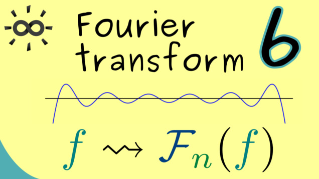
Part 6 - Fourier Series in L²
Now, we are finally ready to define the Fourier series for periodic functions that are integrable over one period. However, we first focus on square-integrable functions because there we have an inner product and the interpretation given by an orthogonal projection. The Fourier series will be denoted by $ n\mapsto \mathcal{F}_n(f) $.
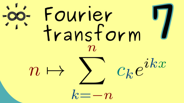
Part 7 - Complex Fourier Series
We already know that trigonometric polynomials can alternatively be represented by complex exponential functions of the form $ e^{i k x} $. However, we didn’t talk how the translation from the cosine and sine functions actually works. Let’s discuss this now and let’s also rewrite the Fourier series in this form. It turns out that everything looks much simple with complex exponential functions.
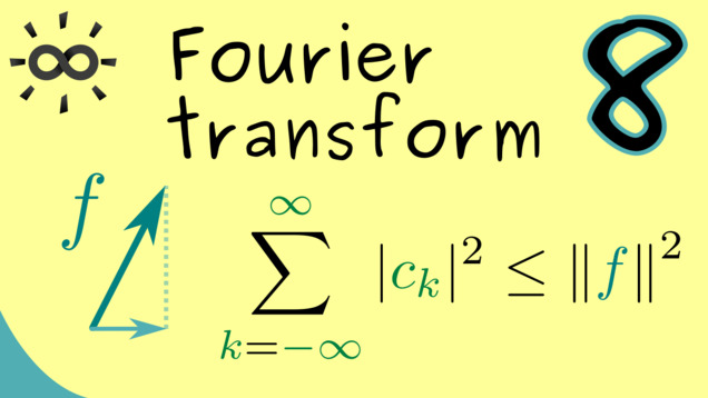
Part 8 - Bessel’s Inequality and Parseval’s Identity
Here, we will discuss some general facts that hold in inner product spaces. Since we have $\mathcal{L}^2$ with our inner product, we can apply the so-called Bessel’s inequality to Fourier series. It turns out that Parseval’s identity is exactly what we want to have for the Fourier coefficients such that the Fourier series converges to the original function.
Part 9 - Total Orthonormalsystem
Let’s quickly discuss equivalent statements to Parseval’s identity, which we can use in later videos. One of them is to say that the orthonormal system we discuss is complete and another is to say that it is total.

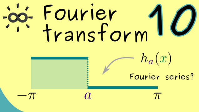
Part 10 - Fundamental Example for Fourier Series
In order to show Parseval’s identity for all square-integrable functions, we first have to look at simple functions, so-called step functions. It turns out that there is a special step functions that can be used as a basis for all step functions, we call it $h_a$ for $a \in [-\pi, \pi]$. Hence, in this video, we first show Parseval’s identity for $h_a$ and this will already make some work.
Content of the video:
00:00 Introduction
00:47 Parseval’s identity for step functions
01:47 Fundamental Step Function
03:42 Fourier Series for Step Function
05:53 Visualization
08:10 Proof of Parseval’s identity
15:37 Credits
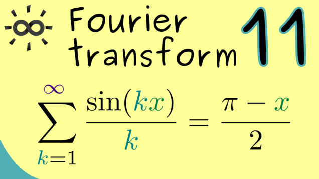
Part 11 - Sum Formulas for Sine and Cosine
This is a technical video where we prove some useful formulas for the theory of Fourier series. One function involved here is often called the Dirichlet kernel but we will not go into it too much. Our goal is to prove the sum formula that we used in the last video. This will be an essential ingredient for our explanation of the theory about approximations with Fourier series.
Content of the video:
00:00 Introduction
01:00 Statement for Cosine Formula
01:51 Note about finite sum of Cosine functions
07:10 Lemma about Sine Formula
08:40 Proof of Lemma
17:13 Visualization of Lemma
18:00 Theorem (Cosine Formula)
18:30 Proof of Theorem
22:22 Applying Weierstrass M-Test
23:57 Find integration constant
25:23 Credits
Part 12 - Parseval’s Identity for Step Functions
Now, we can put everything together and can extend Parseval’s identity to all possible step functions. The key element there is that we have already shown the equality for the special step function $ h_a $. By considering the span of these functions and using some linearity arguments, we can formulate the proof for all step functions.

Part 13 - Fourier Series Converges in L²
After the previous work, we can finally formulate the convergence theorem for $L^2$-functions. Indeed, Parseval’s identity holds for every function $f \in L^2_{per}(\mathbb{R}, \mathbb{C})$ which means that the Fourier series converges with respect to the $L^2$-norm. We will prove this statement by approximating with step functions, for which we already know Parseval’s identity.

Other videos related to this topic:
Part 14 - Uniform Convergence of Fourier Series
At this point, we know that the Fourier Series $ \mathcal{F}_n(f) $ converges to $f$ in the $L^2$-norm. However, this tells us nothing about pointwise convergence at a single point. How can we improve this? It turns out that we can improve it a lot when we consider piecewise $C^1$-functions. There we even have the much stronger uniform convergence, which also includes the pointwise convergence and the $L^2$ convergence. Let’s formulate this theorem and look at an example.

Part 15 - Proof of Uniform Convergence
Now to finish what we have started in the last video: let’s formulate the proof of the theorem about the uniform for piecewise $C^1$-functions. One crucial trick is to use integration by parts for calculating the Fourier coefficients $c_k$ for $k \neq 0$.

Other videos related to this topic:
Part 16 - Calculating Sums with Fourier Series
Since we have the uniform convergence for continuous piecewise $C^1$-function, we can use the Fourier series to evaluate functions at particular points. This can lead to some special sum formulas which might be hard to prove in other ways. In this video, we consider a quadratic function on $[\pi, \pi]$ and extend it $2 \pi$-periodically.

Part 17 - Pointwise Convergence of Fourier Series
Now, let’s finally talk about the pointwise convergence of a Fourier series, even for non-continuous functions. It turns out that we weaken the assumptions from the last videos even more if we just want that the Fourier series convergences pointwisely. We will also find a very nice result. For example, if our function $f$ jumps from 0 to 1 at the origin, then the Fourier series $\mathcal{F}_n(f)(0)$ will converge to $\frac{1}{2}$, assuming that some differential quotients for $f$ exist.

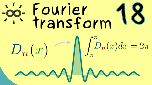
Part 18 - Dirichlet Kernel
In order to prove our latest theorem about the pointwise convergence, we need to talk about the mathematical core behind the Fourier transform. It’s the so-called Dirichlet kernel and we have already talked about it without mentioning the name. Now, we are ready to formulate the crucial properties of it.
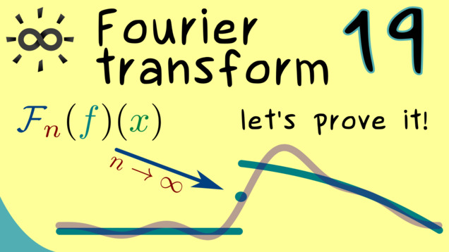
Part 19 - Proof of Pointwise Convergence of Fourier Series
By using the Dirichlet kernel, we can finally write down the proof of the theorem about the point convergence.
Part 20 - Gibbs Phenomenon
We already learnt that we can have uniform convergence for Fourier series, which is a really strong form of convergence. It guarantees that there is no overshooting in any interval for the Fourier series. However, if the original function makes jumps, we simply cannot have a uniform convergence for the Fourier series. Moreover, it turns out that, in this case, we cannot avoid overshooting around the jump point. Gibbs phenomenon tells us that this oscillatory behaviour is always more than 8.9 %. Hence, no matter how large $n$ is, $\mathcal{F}_n(f)$ always has a pointWe already learnt that we can have uniform convergence for Fourier series, which is a really strong form of convergence. It garantuess with this overshooting. Let’s prove this fact for the standard step function:

Part 21 - Fourier Series in L¹
We already mentioned it at the beginning that we can define the Fourier series for periodic $L^1$-functions but we didn’t do it yet because we wanted to use the geometry of the Hilbert space $L^2$. Indeed, we will use all these geometric approaches like orthogonal projections, Parseval’s identity, and so on. So the theory of Fourier series in the general is much more complicated. Let’s have a look at it:

Part 22 - Riemann–Lebesgue Lemma for Fourier Series
Bessel’s inequality already told us that the sequence given by the Fourier coefficients goes to zero when the frequency index tends to $\pm \infty$. However, we already know this for $L^2$-functions because Bessel’s inequality needs the inner product space structure. However, still the results holds for the general case as well and is stated in the famous Riemann–Lebesgue Lemma. We will discuss it and present a proof where Lebesgue’s Dominated Convergence Theorem is used.

Other videos related to this topic:
Part 23 - From Fourier Series to Continuous Fourier Transform
We are finally at the point to leave the periodic functions behind us and talk about the continuous Fourier transform, which is an integral transformation. To motivate it, we will look at $2T$-periodic functions and their Fourier series and look at some limit process $T \rightarrow \infty$. This will justify the general formula we have for the Fourier Transform.

Part 24 - Definition of the Fourier Transform
Let’s leave the $2\pi$-periodic functions behind us and let’s consider integrable functions $f: \mathbb{R}^n \rightarrow \mathbb{C}$. For these functions, the Fourier transform, which we motivated in the last video, is immediately well-defined. We can also show that $\hat{f}$ is a continuous and bounded function by using Lebesgue’s dominated convergence theorem.

Other videos related to this topic:
Part 25 - Example for Fourier Transform
To get the Fourier transform of a given integrable function, we just have to solve one integral for with a parameter $p \in \mathbb{R}^n$. Let’s start with a simple one-dimensional example, which also shows that the Fourier transform does not have to be a $L^1$-function anymore.

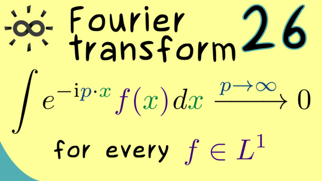
Part 26 - Riemann–Lebesgue Lemma (continuous version)
The Lemma of Riemann-Lebesgue is something we have already discussed in part 22, but there it was formulated for Fourier series. Now, we will extend it to the Fourier transform on $ \mathbb{R}^n $ as well. In particular, this means that the operator $\mathcal{F}$ maps into $C_0(\mathbb{R}^n, \mathbb{C})$, the continuous functions that vanish at infinity.
Other videos related to this topic:
- Multidimensional Integration 11 | Green’s Identities
- Approximation of Integrable Functions with Test Functions
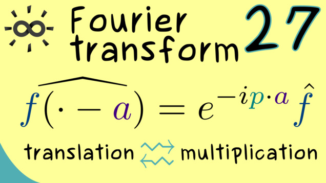
Part 27 - Changes under Translations
Before we dive deeper into the theory of the Fourier transform, we can look at some nice calculation rules we have for this integral transform. In particular, we can consider a translation of an $L^1$-function $f$ and calculate how this influences the corresponding Fourier transform $\hat{f}$. It turns out that such a translation operator is connected to a multiplication operator with a complex exponential function.
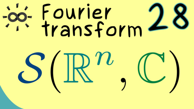
Part 28 - Schwartz Space
To make it easier for us to deal with derivatives in the Fourier transform, we could go to smooth functions. However, it turns out that an even stronger requirement makes the Fourier operator much nicer. We will talk about so-called rapidly decreasing functions, also known as Schwartz functions, named after the French mathematician Laurent Schwartz [lɔʁɑ̃ ʃvaʁts]. For that reason, we denote the vector space by $\mathcal{S}$ and call it the Schwartz space.
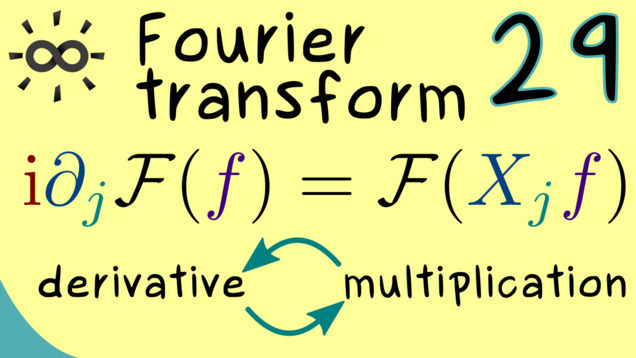
Part 29 - Differentiation and Multiplication Operator
One of the most important properties of the Fourier transform is about what it does with a multiplication operator and a differentiation operator. In short, it will always exchange the rôles. So, for example, the partial differentiation operator $ \partial_j $ will be transformed to $ i M_j$ where $M_j$ just stand for the multiplication with the independent variable $x_j$. This is a really helpful tool to analyze partial differential equations, which we will later see.
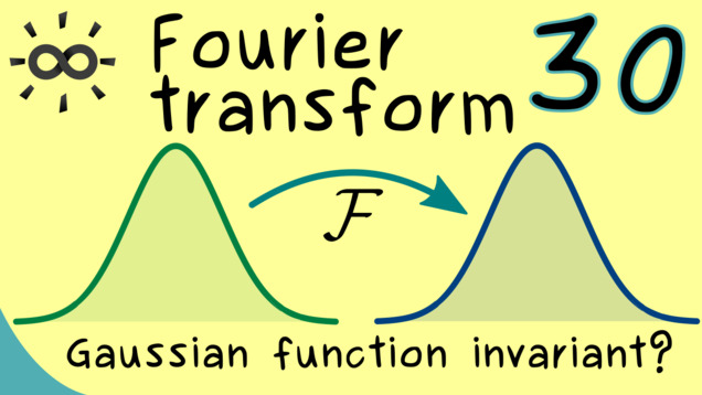
Part 30 - Fixed Point of Fourier Integral Transform
It’s an interesting question if there is a function $f$ which is its own Fourier transform, meaning $\mathcal{F}(f) = f$. Since we have the connection between differentiation and multiplication operators from the last video, we can reduce this question to an ordinary differential equation, which we can solve with standard methods. This will show that the Gaussian function is such a function $f$ that does change under the Fourier transform.
Other videos related to this topic:
- Ordinary Differential Equations 7 | Solving Linear Equations of First Order
- Multidimensional Integration 9 | Integration with Polar Coordinates
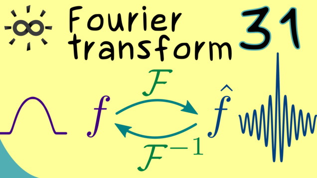
Part 31 - Fourier Inversion Theorem
We can easily show that the Fourier transform maps the Schwartz space $ \mathcal{S}(\mathbb{R}^n, \mathbb{C} ) $ into the Schwartz space again. This justifies that we can apply the Fourier transform to a rapidly descreasing function as many times as we want. In fact, we already see that applying it two times gives almost the original function back. This can be formulated as an inversion formula because it allow to write $f$ as an integral over $\hat{f}$. Let’s prove this formula:
Other videos related to this topic:
- Multidimensional Integration 3 | Fubini’s Theorem
- Measure Theory 10 | Lebesgue’s Dominated Convergence Theorem
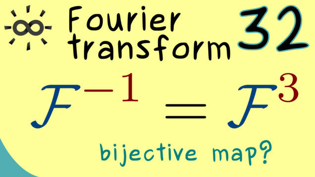
Part 32 - Isomorphism on Schwartz Space
Let’s use the formula from the last video to show that $ \mathcal{F}^4 = \mathrm{id} $ holds on the Schwartz Space $\mathcal{S}(\mathbb{R}^n, \mathbb{C} ) $. This directly shows that the Fourier transform is an isomorphism on this space. However, please always remember, that this does not hold on the whole $L^1$-space. But we can still extend the Fourier inversion theorem to a wider class of integrable functions.
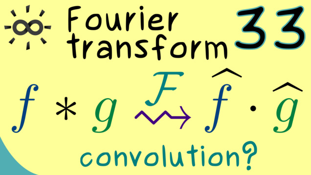
Part 33 - Convolution Theorem
One of the most important properties of the Fourier transform is that it works nicely under the convolution. Please recall that the convolution can be easily defined for $L^1$-functions and it acts like a strange kind of multiplication on the space. Now it turns that the Fourier transform translates the convolution $\ast$ into the ordinary multiplication of functions in the frequency space, in short: $\mathcal{F}( f \ast g) = \mathcal{F}(f) \cdot \mathcal{F}(g)$. However, this formula is not quite correct for common definition of the convolution. In this case the factor $\sqrt{2 \pi}^n$ comes in as well. Let’s see why this is the case:
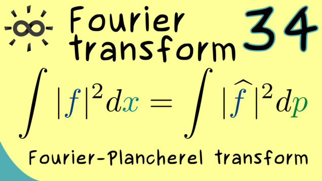
Part 34 - Plancherel Theorem
The Schwartz Space $\mathcal{S}(\mathbb{R}^n)$ becomes an inner product space when we equipp it with the common $L^2$-norm. In fact, this a dense subspace in the Hilbert space $L^2(\mathbb{R}^n)$. This is the key insight to extend the Fourier transform to a unitary operator on this Hilbert space and the resulting operator is sometimes called Fourier-Plancherel transform. In order to do the whole proof, let’s start by showing the isometric property.
Other videos related to this topic:
- Multidimensional Integration 3 | Fubini’s Theorem
- Approximation Theorem 4 | Approximation of Lᵖ-Functions with Test Functions
- Hilbert Spaces 23 | Extension of Isometries
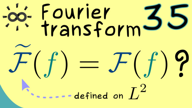
Part 35 - Fourier Transform in L²
The problem with the extension of the Fourier Transform to $L^2$ is that the original formula does not hold in general anymore. However, we can definitely save the formula on the intersection $L^1 \cap L^2$. And from there, we can develop a more general formula that also holds on the whole $L^2$-space.
Other videos related to this topic:
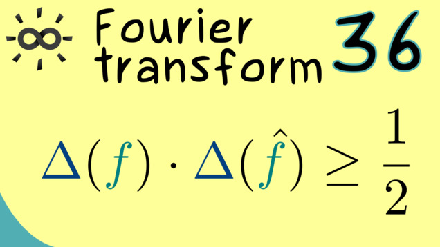
Part 36 - Uncertainty Principle
The uncertainty principle is a core property of the continuous Fourier transform and therefore really relevant in applications. We easily prove it for Schwartz functions if we use multiplication operators $X_j$ and differential operators $P_j$. We find out that the commutator $[P_j, X_j]$ is essentially given by the identity operator. This is the reason for the uncertainty principle, which we can also find in quantum mechanics. Let’s prove it:
Connections to other courses
Summary of the course Fourier Transform
-
You can download the whole PDF here and the whole dark PDF.
-
You can download the whole printable PDF here.
-
Test your knowledge in a full quiz.
- Ask your questions in the community forum about Fourier Transform.
Ad-free version available:
Click to watch the series on Vimeo.