Hello and welcome to my ongoing video course about Ordinary Differential Equations, already consisting of 31 videos. This series explores important concepts in a structured order and is continually updated with new content. Along with the videos, you’ll find helpful text explanations. You can test your knowledge using the quizzes and refer to the PDF versions of the lessons whenever needed. If you have any questions, feel free to ask in the community forum. Let’s dive in!
Part 1 - Introduction
Ordinary Differential Equations is a video series I started for everyone who is interested in the theory of differential equations and dynamics and also in concrete solution methods.:
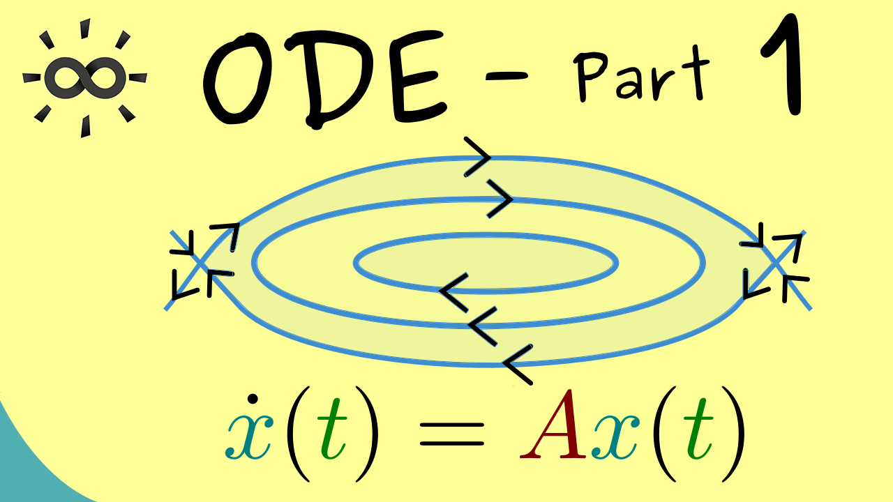
With this you now know the topics that we will discuss in this series. Now, in the next video let us discuss definitions in the topic.
Part 2 - Definitions
There are a lot of notions one has to define to get a precise definition what a differential equation is and what it means to find solutions for it. Let’s do it:

Part 3 - Directional Field
After defining all these new manners of speaking, we are ready to go to a more visual approach. The direction field is essentially just a graph visualisation of a vector-valued function but it helps a lot to get properties from a given differential equation. We will first look at one- and two-dimensional examples.

Part 4 - Reducing to First Order
We already used it in the last video: the fact that every ordinary differential equations could be described as a system of first order. Now we will fill in these gaps and show the correct substitutions, one needs to get this result.

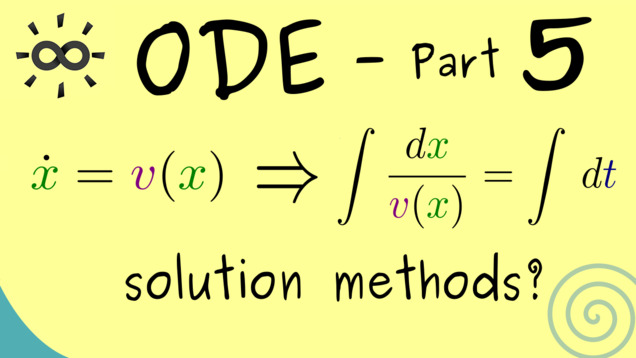
Part 5 - Solve First-Order Autonomous Equations
In this video, we will consider a general one-dimensional differential equation of first order. It turns out that we can describe the solution just as an antiderivate.
Part 6 - Separation of Variables
Now, we are ready to generalise the result from the last video. We can do that in a special situation when two variables can be separated.

Part 7 - Solving Linear Equations of First Order
In this video, we learn about the method of integrating factor to solve linear ODEs. This is equivalent to the method of variation of the constant, which is often taught in this context.

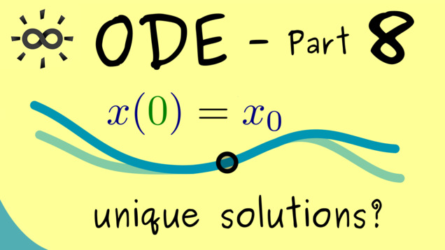
Part 8 - Existence and Uniqueness?
In this video, we start discussing if solutions of initial value problems can exist and if we even find uniquness. By looking at the directional field, we conclude that existence should be given but uniqueness is not garantueed. However, we will give sufficient conditions for unique solutions in future videos.
Part 9 - Lipschitz Continuity
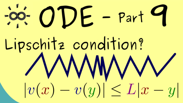
Now, we will look at so-called Lipschitz-continuous functions. They lie, in some sense, between continuously differentiable and continuous functions. It turns out that they give a sufficient criterion for having unique solutions of an initial value problem.
Part 10 - Uniqueness for Solutions
Now we are ready to prove the uniqueness of a solution for a given initial value problem if a Lipschitz condition is satisfied.

Part 11 - Banach Fixed Point Theorem
In order to show the existence for initial value problem, we can use a general result from analysis. This is an important fixed point theorem which can be proven just by just using some knowledge of convergent sequences and complete spaces. However, I don’t want to show proof but how to apply to ordinary differential equations.
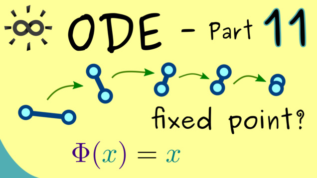
If you want to learn how to proof this important theorem, you can check out the supplementary video about the Banach fixed-point theorem.
Part 12 - Picard–Lindelöf Theorem
Finally, we can state the famous Picard–Lindelöf Theorem, which summarizes existence and uniqueness for an inital value problem assuming the corresponding vector field is Lipschitz-continuous.
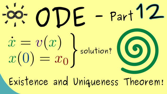
Content of the video:
00:00 Introduction
00:51 Initial value problem
01:12 Assumption: locally Lipschitz continuous function
01:48 Banach fixed-point theorem
02:18 Define metric space and contraction
03:51 Function Space X
04:43 Correction: codomain of α has to be changed, see PDF
07:39 Complete metric function space
08:10 Check the contraction
12:08 Correction: new codomain of α needed, see PDF
12:53 Make epsilon small enough
13:09 Picard-Lindelöf theorem
14:26 Credits
Other videos related to this topic:
Part 13 - Picard Iteration
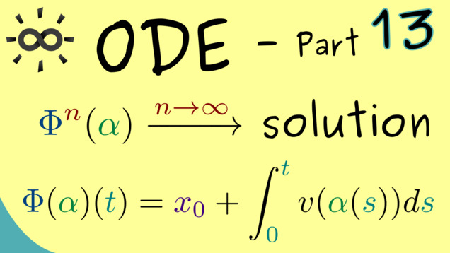
The proof of the Picard–Lindelöf Theorem used the Banach fixed-point theorem. However, this one comes with an interation formula for approximating the fixed-point. It’s a general result and therefore also useful in the theory of ordinary differential equations. Indeed, we can start with an approximation of the solution for an initial-value problem and then we can improve it step by step. In the limit we get the actual unique solution. This whole procedure, which only includes integration, is known as the Picard iteration.
Part 14 - Maximal and Global Solutions
Now, we have to get more technical. For always talked about uniqueness in the local sense. We just showed that in a small neighbourhood the solution of an initial value problem has to be unique. However, how is it in a global sense? Can we extend this local behaviour to a larger domain? To answer this, we have to define the notions maximal solution and global solution.
Part 15 - Phase Portrait
Before we already mentioned the phase space for an ordinary differential equation. We could sketch the directional field for a system $ \dot{x} = v(x) $ and also so-called orbits. Now, the collection of all these orbits gets a special: we call it the phase portrait. For locally Lipschitz continuous vector field, we have the result that orbits fill out the whole picture and that two orbits cannot cross each other.

Part 16 - Periodic Solutions and Fixed Points
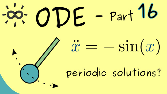
Let’s look at some special orbits we find in the phase potrait: fixed points and periodic solutions. To visualize these special solutions, let’s consider the mathematical pendulum given by the ordinary differential equation $ \ddot{x} = - \sin(x) $.
Part 17 - Picard–Lindelöf Theorem (General and Special Version)
Let’s revisit the Picard-Lindelöf theorem again. We can generalize the claim to non-autonomous systems where we only need a suitable Lipschitz condition in the space-variable, and we can also specify the theorem if we have a global Lipschitz condition instead of a local one. In the last case, we can prove the existence of global solutions.

Part 18 - System of Linear Differential Equations
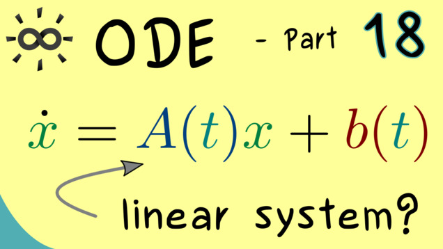
In part 7, we already discussed how to solve linear differential equations, but this was restricted to the one-dimensional case. So it’s a natural question to ask if one can generalize this whole procedure to an $n$-dimensional system. This is one is written as $\dot{x} = A(t) x + b(t)$ where $ A(t) \in \mathbb{R}^{n \times n} $.
Part 19 - Solution Space
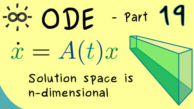
Let’s consider the homogenous part of system of linear ODEs. For this, we can prove that the set of solutions forms a vector space. Moreover, we are also able to calculate the dimension of this solution space.
Part 20 - Matrix Exponential
It turns out that we can make sense of $e^A$ where $A$ is matrix. This generalizes the idea of finding solution for a one-dimensional ODE of the form $ \dot{x} = a x $, where the solution space is spanned by $ t \mapsto e^{a t} $. In this video, we will show that, for a homogeneous and autonomous system $ \dot{x} = A x $, the solution space is also spanned by the columns of the matrix $ e^{t A} $.

Other videos related to this topic:
Part 21 - Solution Set of Linear ODEs
To generalize the discussions from the last videos, we can finally explain how the solution set for a general system of linear ODEs looks like. It turns out that the homogenous part contains almost already all information.

Part 22 - Properties of the Matrix Exponential
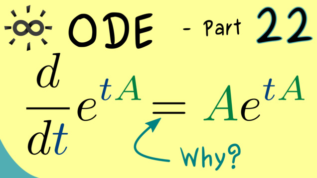
We’ve already seen that the matrix exponential represents the solution set of an autonomous linear ODE. Therefore, it’s important that we know how to calculate with an expression like $e^{t A}$. In particular, we want to know what the derivative of the function $t \mapsto e^{t A}$ is and when the formula $e^{A+B} = e^{A} \cdot e^{B} $ holds.
Part 23 - Example for Matrix Exponential
After a lot of theoretical discussions, we can finally look at an explicit calculation of a matrix exponential to solve a system of linear differential equations. The important thing is that we have an autonomous system such we can easily calculate the matrix exponential. It turns out that, in particular for diagonalizable matrices, this construction is straightforward. One just has to determine eigenvalues and eigenvectors to calculate all the powers of the given matrix $A$.

Part 24 - Characteristic Polynomial
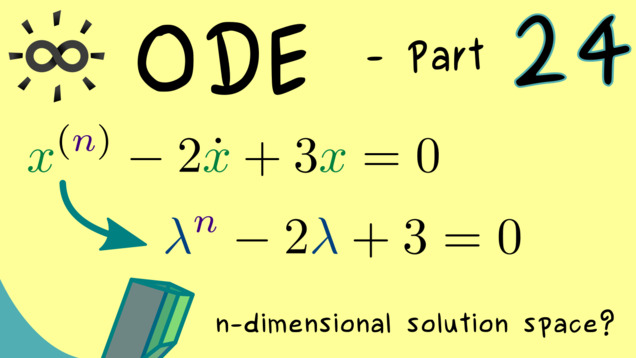
Let’s look at higher order ODEs again. In particular, linear differential equations can be solve with our method from first order systems, which means by using the matrix exponential. There, we already know that the key ingeredient is given by eigenvalues and therefore by the zeros of the characteristic polynomial. It turns out that we can also directly define it for a linear differential equation of order $n$.
Part 25 - Example for Non-Diagonalizable Matrix
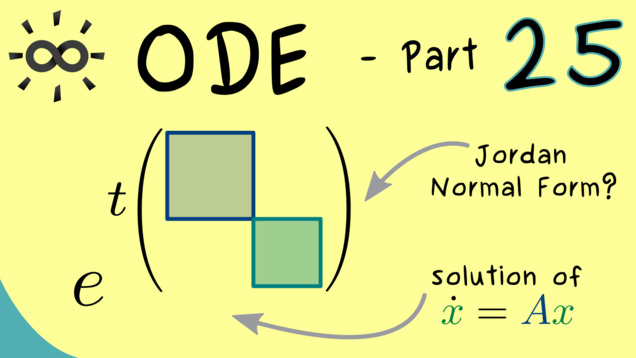
We explain the general approach to calculate $e^{t A}$ for every complex matrix $A$. To understand this, it might be really helpful to see an explicit example first. That is what we do in this video.
Part 26 - Two-Dimensional Solution Spaces
We already know that the columns of $\exp(t A)$ span the solution set of $\dot{x} = A x$. So it’s not hard at all to calculate all possible cases that can happen for a two-dimensional system. Indeed, this knowledge is also helpful to understand what can happen for higher-dimensional systems.

Part 27 - Solutions of Linear Second-Order ODE
Since we can transform every linear ODE into a system of first order, we can use the solution theory from the last video to completely solve the second-order autonomous case. In fact, not all cases of a two-dimensional system can occur in this situation. Let’s examine this in more detail.

Part 28 - Wronski Determinant
Let’s go back to a general system of linear ODES: $\dot{x} = A(t) x + b(t)$. We already know that we need to find the $n$-dimensional solution space of the homogeneous system and one particular solution to get the whole solution set. Since we don’t have an autonomous system here, the matrix exponential will not help. A good substitute for this is a so-called fundamental matrix solution, and the determinant of it is called Wronskian or Wronski determinant.

Part 29 - Liouville’s Formula
Defining the Wronksi determinant from the last video had a practical value: it can determine if a set of solutions are linearly independent and span the whole solution space. One possibility to show this is to use Liouville’s Formula, also known as Abel’s identity. We will see that it comes out as a solution from a one-dimensional ODE.

Other videos related to this topic:
Part 30 - Method Of Integrating Factors
The method of integrating factors for linear ODEs was already discussed in part 7. Now, we try to extend this formula to the general $n$-dimensional case. In order to do this, we will define principal matrix solution of the homogeneous system, denoted by $\Pi(t)$.

Part 31 - D’Alembert Reduction
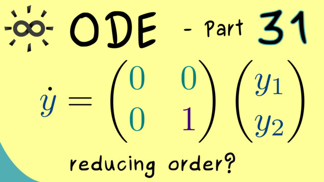
After a lot of theoretic explanations, we should eventually look at a concrete example of a $2\times 2$ linear system of ODEs. Unfortunately, there is no general recipe to solve a non-autonomous linear system, but it’s always possible to reduce the order (or dimension) of the system if we already know one solution. This is often know as reduction of order or d’Alembert reduction. Especially for $2\times 2$-system is a valid strategy to find the second linearly independent solution. Let’s discuss how this works.
Summary of the course Ordinary Differential Equations
-
You can download the whole PDF here and the whole dark PDF.
-
You can download the whole printable PDF here.
- Ask your questions in the community forum about Ordinary Differential Equations.
Ad-free version available:
Click to watch the series on Vimeo.