-
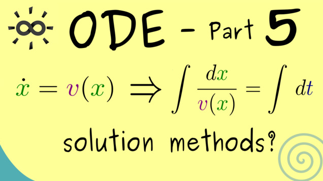
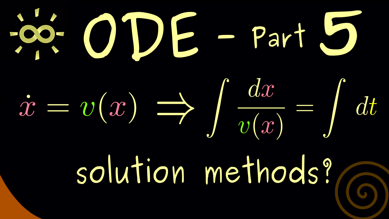
Title: Solve First-Order Autonomous Equations
-
Series: Ordinary Differential Equations
-
Chapter: Solving Strategies
-
YouTube-Title: Ordinary Differential Equations 5 | Solve First-Order Autonomous Equations
-
Bright video: Watch on YouTube
-
Dark video: Watch on YouTube
-
Ad-free video: Watch Vimeo video
-
Forum: Ask a question in Mattermost
-
Quiz: Test your knowledge
-
Dark-PDF: Download PDF version of the dark video
-
Print-PDF: Download printable PDF version
-
Thumbnail (bright): Download PNG
-
Thumbnail (dark): Download PNG
-
Subtitle on GitHub: ode05_sub_eng.srt
-
Download bright video: Link on Vimeo
-
Download dark video: Link on Vimeo
-
Timestamps (n/a)
-
Subtitle in English
1 00:00:00,443 –> 00:00:04,633 Hello and welcome back to ODEs.
2 00:00:04,833 –> 00:00:09,787 The video series where we solve such equations and talk about the theory behind it.
3 00:00:09,987 –> 00:00:16,101 Indeed in today’s part 5 we will talk about solving strategies for autonomous equations.
4 00:00:16,301 –> 00:00:21,886 More precisely we will have a first order, autonomous ODE in one dimension
5 00:00:22,214 –> 00:00:27,589 and in fact it turns out that we have a general solving method for these equations.
6 00:00:28,214 –> 00:00:36,106 However before we start with the details, I first want to thank all the nice people who support this channel on Steady, via PayPal or by other means
7 00:00:36,743 –> 00:00:43,418 and you might already know, as a reward for supporting me you get PDF versions and quizzes for all the videos.
8 00:00:43,771 –> 00:00:49,583 Just use the link in the description to find my web page and there you can download everything.
9 00:00:50,257 –> 00:00:54,029 Ok, then without further ado let’s start with the topic of today
10 00:00:54,043 –> 00:00:58,833 by first discussing what we mean, when we talk about an initial value problem.
11 00:00:59,400 –> 00:01:07,323 The name already tells you, we want to find some special solutions for a differential equation that satisfies some initial condition.
12 00:01:07,943 –> 00:01:12,686 More concretely it means, first we have our first order differential equation
13 00:01:12,771 –> 00:01:19,705 given as “x dot” is equal to v(x), where v should be a continuous function.
14 00:01:20,471 –> 00:01:25,851 We already talked about that this is the general form of ODEs, like we want to consider them.
15 00:01:26,051 –> 00:01:29,697 However now we want to restrict that to one dimension.
16 00:01:29,897 –> 00:01:35,304 In other words it’s not a system, it’s just one ODE
17 00:01:36,086 –> 00:01:42,428 and to make it simpler, the function v should be defined on the whole real number line and a continuous function
18 00:01:42,886 –> 00:01:50,743 and now the initial value is stated as: x at the position 0 is equal to a given value x_0.
19 00:01:51,386 –> 00:01:55,973 So you see x_0 here is just a given real number
20 00:01:56,173 –> 00:02:02,363 and now solving this initial value problem means that we want to find all solutions alpha
21 00:02:02,629 –> 00:02:11,384 and such a solution could be defined on any interval (t_0, t_1), but it’s important that at least the point 0,
22 00:02:11,443 –> 00:02:15,210 the point in time 0 lies inside this interval.
23 00:02:15,871 –> 00:02:23,378 Now, as a reminder solutions simply means: if you put the function alpha into the ODE, it solves it.
24 00:02:23,578 –> 00:02:32,147 In other words alpha dot(t) is equal to v(alpha(t)) for all t in the interval t_0 to t_1.
25 00:02:32,347 –> 00:02:41,856 However for solving the initial value problem we want more. We also want that alpha at the point 0 is equal to x_0.
26 00:02:42,056 –> 00:02:46,922 This means that we fix the value of the solution at a given time point
27 00:02:47,429 –> 00:02:52,653 and please note that this point is chosen as 0, is not a restriction at all.
28 00:02:52,853 –> 00:02:58,325 Simply because we have an autonomous ODE, where the time is not explicitly in it.
29 00:02:58,525 –> 00:03:04,363 This means 0 here is an arbitrary choice, but it is without lost of generality.
30 00:03:04,563 –> 00:03:11,056 Ok and now the question is: “how can we solve such an ODE with a given initial condition?”
31 00:03:11,256 –> 00:03:16,349 and indeed, there is a general solving strategy we now can develop.
32 00:03:16,657 –> 00:03:23,478 However let’s first do that in the case that v at our value x_0 is not 0.
33 00:03:23,900 –> 00:03:29,169 In other words this value here should be strictly positive or strictly negative.
34 00:03:29,871 –> 00:03:36,937 We take this case, because there we can simplify the ODE by dividing by v(x).
35 00:03:37,800 –> 00:03:44,029 Hence the ODE now looks like that. x dot divided by v(x) is equal to 1.
36 00:03:44,229 –> 00:03:51,714 Please note, because v is a continuous function this whole thing here makes sense in the neighbourhood around x_0.
37 00:03:52,429 –> 00:04:01,380 This means that the function v could have 0 and it would make problems here. However in some sense they are far off, of x_0.
38 00:04:01,580 –> 00:04:06,882 Therefore only around x_0 we consider the ODE in this form.
39 00:04:07,082 –> 00:04:17,608 Therefore now we know: any solution alpha here with the condition that 0 is in the domain and alpha(0) = x_0 fulfills the following
40 00:04:17,808 –> 00:04:25,020 By definition we have alpha dot(s) divided by v(s) is equal to 1
41 00:04:25,220 –> 00:04:33,373 and you already see, we use s as the independent variable here, because we want to use t for something else later.
42 00:04:33,573 –> 00:04:39,900 Therefore to make this precise we would say this equation holds for all s in the given interval
43 00:04:40,100 –> 00:04:47,215 and now you might already guess. In order to solve this equation now, we will integrate on both sides
44 00:04:48,000 –> 00:04:53,171 and namely we will simply integrate from the given point 0 to a given point t.
45 00:04:53,514 –> 00:04:58,325 Hence on the right-hand side it simply means that we get out t.
46 00:04:58,525 –> 00:05:03,593 We integrate a constant from 0 to t. So the result would be t
47 00:05:03,793 –> 00:05:10,982 and now please note, that holds for all possible t and you can also go backwards to the original equation.
48 00:05:11,586 –> 00:05:18,705 So you would say this is simply differentiating and then you get the result with the fundamental theorem of calculus.
49 00:05:18,905 –> 00:05:24,871 Indeed, this is a very important result that we need to solve ODEs
50 00:05:25,586 –> 00:05:30,900 and if you don’t know it, please check out my real analysis series, where we also prove it.
51 00:05:31,100 –> 00:05:35,699 Moreover in real analysis we also learn how to deal with integrals.
52 00:05:35,899 –> 00:05:41,585 For example we know we can use the substitution rule to solve such an integral here
53 00:05:41,900 –> 00:05:45,719 and in fact this will be exactly our next step here
54 00:05:46,543 –> 00:05:52,525 and there we should immediately see that it helps to introduce a new variable x for alpha(s)
55 00:05:52,725 –> 00:06:02,027 and now by knowing the substitution rule, you know informally that we can write dx = alpha dot(s) ds
56 00:06:02,227 –> 00:06:08,791 and then these 2 things here are exactly the 2 things we will substitute here inside the integral.
57 00:06:09,329 –> 00:06:13,694 In other words we have the integral of 1 divided by v(x)
58 00:06:14,157 –> 00:06:21,070 and then most importantly don’t forget the boundaries. Now we integrate from alpha(0) to alpha(t).
59 00:06:21,614 –> 00:06:28,270 However we already know alpha(0) is equal to our initial value x_0.
60 00:06:28,643 –> 00:06:34,187 Therefore let’s immediately pull that in instead of alpha(0) we now write x_0.
61 00:06:34,743 –> 00:06:41,878 Moreover the right-hand side is not changed at all. We still have that this integral is equal to t for all t.
62 00:06:42,078 –> 00:06:52,188 Ok and with that we see in order to solve our original ODE we have to find antiderivatives of the function 1 divided by v.
63 00:06:52,388 –> 00:06:58,033 So again we recognize that the fundamental theorem of calculus goes in here,
64 00:06:58,233 –> 00:07:04,397 because from that we can conclude that an integral can be written with antiderivatives.
65 00:07:04,597 –> 00:07:12,557 More precisely we have the antiderivative at the upper limit, alpha(t) - the antiderivative at the lower limit
66 00:07:12,855 –> 00:07:16,935 and in this case we already know this is simply x_0.
67 00:07:17,586 –> 00:07:26,960 So there we see we have our new equation here and please don’t forget. Capital F should be an antiderivative of the function 1/v.
68 00:07:27,160 –> 00:07:34,964 This means that this procedure here only works if we are able to find an antiderivative of the function 1/v.
69 00:07:35,271 –> 00:07:40,987 However in the case that we are able to do that, the ODE is almost solved
70 00:07:41,187 –> 00:07:49,271 and maybe in order to see that, let’s call F(x_0) just c. So it’s just any constant here in this equation.
71 00:07:49,886 –> 00:07:54,425 Therefore in our next step let’s put this constant to the right-hand side
72 00:07:55,200 –> 00:08:01,218 and then we see the solution we search for, alpha(t), is almost on the left-hand side.
73 00:08:02,029 –> 00:08:07,192 In fact we just have to find the inverse of F to isolate alpha(t)
74 00:08:07,392 –> 00:08:14,216 and there I can already tell you this is always possible by our assumption around our value x_0.
75 00:08:14,416 –> 00:08:20,466 In other words locally we don’t have a problem finding an inverse function of F
76 00:08:20,666 –> 00:08:25,527 and in conclusion that is all we need for solving our ODE.
77 00:08:25,727 –> 00:08:31,124 So on the right we simply have F inverse of t minus our constant c.
78 00:08:32,129 –> 00:08:36,899 So in summary we can say we find a solution of our ODE by doing that
79 00:08:37,099 –> 00:08:42,972 and then we simply have to adjust the constant such that our initial value is also satisfied
80 00:08:43,714 –> 00:08:50,586 and with that we have it. This is the whole procedure of solving an autonomous ODE of first order.
81 00:08:51,286 –> 00:08:59,181 Now, of course the problem is that this looks theoretical. So I want to show you 2 examples and how we can apply this procedure
82 00:08:59,557 –> 00:09:04,343 and there we will also see that you don’t have to memorize the procedure from above.
83 00:09:04,443 –> 00:09:07,103 You simply have to know what to do in the calculation.
84 00:09:07,857 –> 00:09:13,717 Now let’s say we have the ODE x dot is equal to lambda times x, with a positive lambda
85 00:09:13,917 –> 00:09:18,611 and then for the initial condition we assume that x_0 is not 0,
86 00:09:19,329 –> 00:09:23,039 because in this case we can use our procedure from above.
87 00:09:23,829 –> 00:09:31,164 Ok and in this point I want to show you an informal step that helps you to memorize the procedure from above.
88 00:09:31,457 –> 00:09:39,140 So we rewrite the derivative x dot as dx/dt and then we informally multiply with dt.
89 00:09:39,340 –> 00:09:45,006 It seems strange, but it brings us to the correct form, we have already justified above.
90 00:09:45,206 –> 00:09:51,765 So the idea is to bring everything with x to the left-hand side and everything with t to the right-hand side.
91 00:09:52,171 –> 00:09:56,433 In other words we have lambda times dt on the right-hand side now
92 00:09:57,129 –> 00:10:01,351 and then we simply write an integral sign on both sides,
93 00:10:01,743 –> 00:10:06,037 because then the separated dx and dt makes sense again
94 00:10:06,429 –> 00:10:13,476 and then you should see on the left this is just a short notation for the antiderivative of 1/v.
95 00:10:13,800 –> 00:10:19,106 Of course not completely, because the constant we already put on the other side.
96 00:10:19,386 –> 00:10:27,173 However of course this is not a problem, because we already know on the right-hand side we just have t with a constant anyway.
97 00:10:27,914 –> 00:10:34,151 Ok and now this equation says we have to write antiderivatives on the left-hand side and on the right hand side
98 00:10:34,529 –> 00:10:41,557 and the antiderivative of 1/x is given by the natural logarithm of the absolute value of x
99 00:10:42,129 –> 00:10:46,638 and on the right hand side we just have lambda as t, as we already know it.
100 00:10:47,457 –> 00:10:55,031 However please don’t forget, before there was a constant involved, because of the value of the antiderivative at x_0.
101 00:10:55,514 –> 00:11:00,584 In fact different antiderivatives only differ by an additive constant.
102 00:11:01,400 –> 00:11:07,194 This means we can just deal with that fact by adding a constant here in the equation.
103 00:11:07,629 –> 00:11:15,969 I call it capital C and the idea as before is that we find the correct constant such that our initial value is satisfied.
104 00:11:16,343 –> 00:11:21,686 So that’s what you should see. It does not matter if we use this -c here or this +C here.
105 00:11:21,786 –> 00:11:25,928 It’s all the same. We just have to find the correct constant in the end
106 00:11:26,286 –> 00:11:31,194 and usually we just shift that problem to the end of the whole calculation.
107 00:11:31,394 –> 00:11:38,277 Ok and then you already know in the next step we have to apply the inverse function of the natural logarithm here
108 00:11:39,000 –> 00:11:43,158 and there you should know this is given by the exponential function.
109 00:11:43,914 –> 00:11:49,202 So we have e to the power lambda times t, times e to the power of constant C
110 00:11:49,402 –> 00:11:55,598 and of course this x in the left-hand side here should now be our solution alpha(t).
111 00:11:55,798 –> 00:12:00,127 So in order to make that clear now we should also use this notation
112 00:12:00,327 –> 00:12:04,802 and then you see the only thing that remains is that we have an absolute value here.
113 00:12:05,002 –> 00:12:09,608 Which means either we have +the right-hand side or -the right-hand side
114 00:12:10,557 –> 00:12:14,721 and with these 2 cases we have solved our initial value problem.
115 00:12:14,921 –> 00:12:18,170 So please note, e of something is always positive.
116 00:12:18,370 –> 00:12:23,385 So either we have a completely negative solution or a function that is always positive
117 00:12:23,929 –> 00:12:32,955 and now by putting in t is equal to 0 to find our x_0, we also get that this constant in front should be x_0.
118 00:12:33,155 –> 00:12:40,646 In other words the solution is then very short. It’s simply x_0 times exponential function of lambda times t.
119 00:12:41,371 –> 00:12:45,686 Now, this whole thing here is a standard, but also a very important example
120 00:12:45,814 –> 00:12:49,900 and you see, now we have found all the solutions in this form.
121 00:12:50,129 –> 00:12:55,565 So for this example we can also say something about the uniqueness of solutions.
122 00:12:56,300 –> 00:13:02,173 So this is already very good, but of course in general we will talk about this issue later.
123 00:13:02,843 –> 00:13:08,628 First here I want to show you another example. Namely x dot is equal to x squared
124 00:13:08,828 –> 00:13:14,960 and as before our initial condition is given as x_0 not equal to 0
125 00:13:15,160 –> 00:13:21,318 and now as we have learned before we can do exactly the same steps as in the example above.
126 00:13:22,029 –> 00:13:27,390 Indeed, we already know this whole separation idea gives us the correct form in the end.
127 00:13:28,057 –> 00:13:35,164 So on the left we have dx/x^2 and on the right we just have dt
128 00:13:35,686 –> 00:13:41,039 and now as before we write an integral to get antiderivatives into the game.
129 00:13:41,239 –> 00:13:50,527 So the antiderivative on the left hand side is just -1/x and on the right-hand side it’s just t as always.
130 00:13:50,727 –> 00:13:59,186 However as before, please don’t forget to add a constant, because this is needed to actually solve our initial value problem
131 00:13:59,386 –> 00:14:05,640 or to put it in other words we want to find a general form of the solution and now just 1 particular solution.
132 00:14:06,429 –> 00:14:10,233 Therefore please in this step never forget the constant!
133 00:14:10,971 –> 00:14:18,098 Ok and now as before in order to make it consistent with our notation, let’s use alpha(t) now instead of just x
134 00:14:18,957 –> 00:14:25,973 and then in the next step we just have to take the inverse here, to get alpha(t) on the left-hand side alone.
135 00:14:26,386 –> 00:14:33,410 Now this is not hard to see. How solution alpha(t) is -1/(t+C).
136 00:14:34,200 –> 00:14:43,495 So this is the general form of the solution and now we just have to find what the constant C is, in order to satisfy our initial value.
137 00:14:43,695 –> 00:14:48,701 So this is no problem at all. We simply put in 0, into our form here
138 00:14:49,129 –> 00:14:54,209 and then we see we have -1/C
139 00:14:54,286 –> 00:14:59,168 and now we know by our initial value problem that this should be equal to x_0.
140 00:15:00,029 –> 00:15:03,752 Hence we have an equation that we can solve for C
141 00:15:03,952 –> 00:15:09,886 and this is not a problem at all. C is simply given by -1/x_0
142 00:15:10,643 –> 00:15:16,124 and that’s exactly the thing we have to put into our general form here
143 00:15:16,914 –> 00:15:22,274 and then indeed, we can state the solution of our initial value problem here.
144 00:15:22,614 –> 00:15:30,476 So it’s alpha(t) is equal to -1/(t+(-1/x_0))
145 00:15:30,900 –> 00:15:35,350 and now of course we can simplify that by expanding the fraction.
146 00:15:35,550 –> 00:15:41,933 There we have x_0/(1-x_0 times t)
147 00:15:42,586 –> 00:15:47,646 and there you see this is the solution. We have solved our initial value problem.
148 00:15:48,471 –> 00:15:56,252 Ok and with that we have seen some nice examples and I would say in the next video let’s go deeper into the theory again.
149 00:15:57,043 –> 00:16:00,696 So I really hope that I see you there and have a nice day. Bye!
-
Quiz Content
Q1: Consider the ordinary differential equation $\dot{x} = \sin(x)$. Is there a solution for the initial value problem with $x(0) = 1$?
A1: Yes, because $\sin(1) \neq 0$ and the solving strategy from the video works.
A2: No, because $\sin(0) = 0$ and the solving strategy from the video does not work.
A3: No, because calculating the antiderivative is not possible.
Q2: Consider the ordinary differential equation $\dot{x} = x^{-1}$. What is a solution for initial value problem with $x(0) = 1$?
A1: $\alpha(t) = \sqrt{ 2 t + 1} $
A2: $\alpha(t) = -\sqrt{ 2 t + 1} $
A3: $\alpha(t) = \sqrt{ 2 t} $
A4: $\alpha(t) = - \sqrt{ 2 t} $
A5: $\alpha(t) = \frac{1}{t+1} $
-
Last update: 2025-08