
-
Title: Definition of the Fourier Transform
-
Series: Fourier Transform
-
Chapter: Continuous Fourier Transform
-
YouTube-Title: Fourier Transform 24 | Definition of the Fourier Transform
-
Bright video: Watch on YouTube
-
Dark video: Watch on YouTube
-
Ad-free video: Watch Vimeo video
-
Forum: Ask a question in Mattermost
-
Dark-PDF: Download PDF version of the dark video
-
Print-PDF: Download printable PDF version
-
Thumbnail (bright): Download PNG
-
Thumbnail (dark): Download PNG
-
Subtitle on GitHub: ft24_sub_eng.srt
-
Download bright video: Link on Vimeo
-
Download dark video: Link on Vimeo
-
Related videos:
-
Timestamps (n/a)
-
Subtitle in English
1 00:00:00.605 –> 00:00:01.915 Hello and welcome back
2 00:00:01.915 –> 00:00:04.235 to Fourier Transform the video series
3 00:00:04.245 –> 00:00:06.835 where we talk a lot about Fourier analysis,
4 00:00:07.135 –> 00:00:09.955 in particular the continuous Fourier transform.
5 00:00:10.615 –> 00:00:12.475 And indeed in today’s part 24,
6 00:00:12.695 –> 00:00:14.635 we will finally give the definition
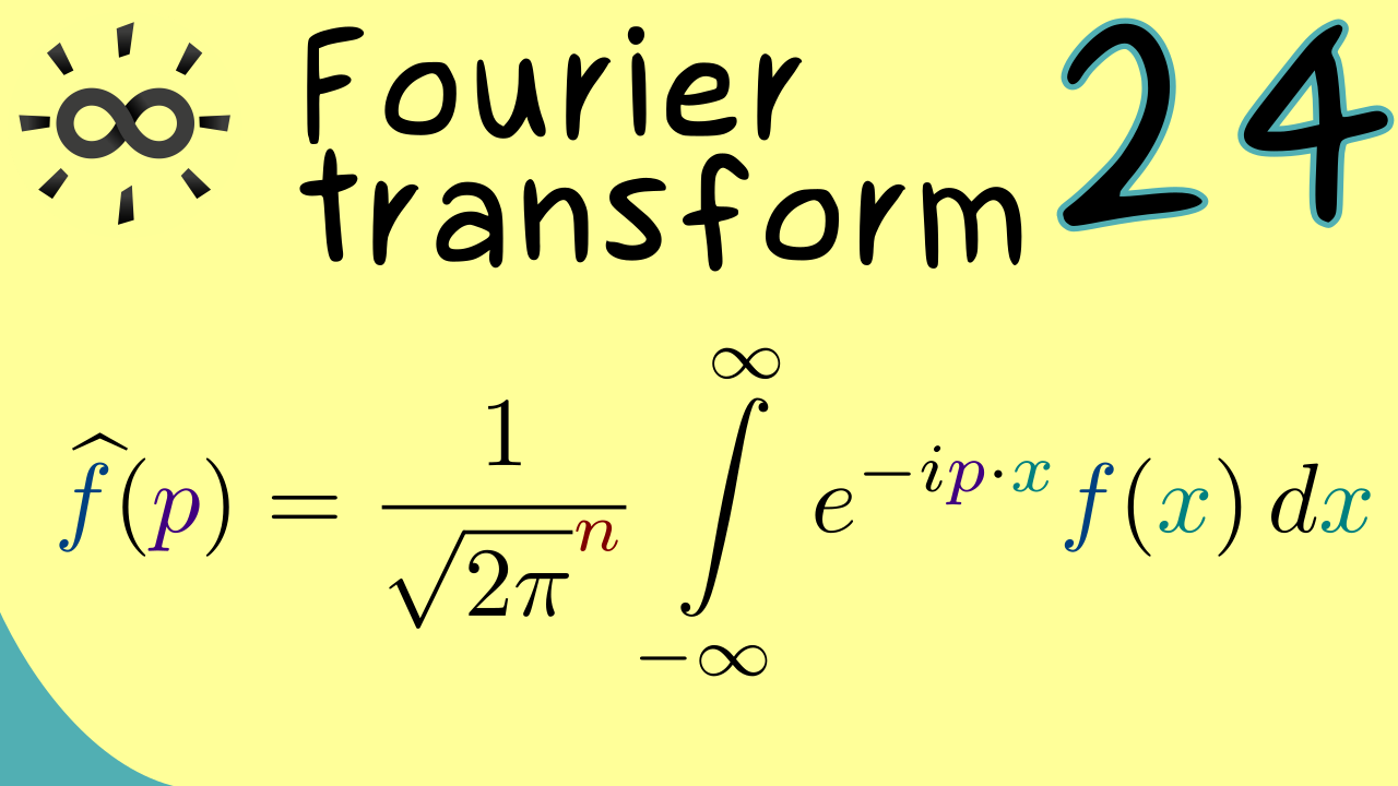
7 00:00:14.695 –> 00:00:17.915 for the Fourier transform as an integral transformation.
8 00:00:18.485 –> 00:00:20.775 However, before we do that, I first want
9 00:00:20.775 –> 00:00:22.095 to thank all the nice people
10 00:00:22.115 –> 00:00:24.055 who support this channel on Steady here, on
11 00:00:24.055 –> 00:00:25.375 YouTube, or via other means.
12 00:00:26.155 –> 00:00:28.535 And please don’t forget, as a Steady member, you get a lot
13 00:00:28.535 –> 00:00:31.855 of rewards like PDF versions, quizzes, and books.
14 00:00:32.525 –> 00:00:35.055 Just click the link in the description to download them.
15 00:00:35.875 –> 00:00:39.455 And then I would say we can immediately start with the definition
16 00:00:39.475 –> 00:00:40.895 of the Fourier transform.
17 00:00:41.475 –> 00:00:43.615 In the last video, we have already discussed
18 00:00:43.615 –> 00:00:46.935 how this definition should look like when we come from the
19 00:00:46.935 –> 00:00:50.125 Fourier series, and now we will extend this
20 00:00:50.265 –> 00:00:53.405 to all integrable functions defined on Rn
21 00:00:54.075 –> 00:00:57.605 more precisely we work in L one, which is a space
22 00:00:57.625 –> 00:01:01.285 of equivalence classes of Lebesgue integrable functions on Rn.
23 00:01:01.345 –> 00:01:04.565 The most important part for us is
24 00:01:04.565 –> 00:01:07.365 that this is a vector space with a norm.
25 00:01:08.145 –> 00:01:12.125 And in that sense the Fourier transform is a linear map.
26 00:01:12.945 –> 00:01:16.285 And I will denote this abstract map by a curved F.
27 00:01:16.985 –> 00:01:19.725 And as already mentioned, the input space is given
28 00:01:19.785 –> 00:01:21.765 by the Lebesgue integrable functions.
29 00:01:22.485 –> 00:01:25.695 However, the best choice for the output space, we don’t know
30 00:01:25.755 –> 00:01:28.455 yet, but we can choose it as large as we can
31 00:01:28.685 –> 00:01:31.895 with the function space of functions defined on Rn.
32 00:01:32.395 –> 00:01:35.335 So the Fourier transform will definitely map into this
33 00:01:35.335 –> 00:01:37.975 space, but we will show in this video already
34 00:01:38.165 –> 00:01:39.735 that we can make it much smaller.
35 00:01:40.515 –> 00:01:43.655 In fact, the image of a function f under the Fourier
36 00:01:44.015 –> 00:01:45.055 transform denoted
37 00:01:45.075 –> 00:01:48.655 by f hat is always a continuous function on Rn.
38 00:01:49.235 –> 00:01:50.695 So you can already remember that.
39 00:01:50.915 –> 00:01:52.415 But before we can prove it,
40 00:01:52.555 –> 00:01:55.695 we should first write down the definition of f hat.
41 00:01:56.355 –> 00:01:59.575 And in the following, I will always use the variable name p
42 00:01:59.915 –> 00:02:01.535 for the functions on the right hand side.
43 00:02:02.155 –> 00:02:05.175 On the other hand, the functions on the left hand side will
44 00:02:05.175 –> 00:02:06.495 get the variable name x.
45 00:02:07.435 –> 00:02:08.935 Now at this point, you should already know
46 00:02:08.935 –> 00:02:12.455 that the Fourier transform is an integral transformation.
47 00:02:13.115 –> 00:02:15.575 And for the reasons we have discussed in the last video,
48 00:02:15.875 –> 00:02:18.215 we have a constant in front of this integral.
49 00:02:18.925 –> 00:02:22.535 It’s one over the square root of two pi to the power n.
50 00:02:23.115 –> 00:02:25.895 So the dimension of our space Rn also
51 00:02:25.895 –> 00:02:27.335 goes into the constant.
52 00:02:28.235 –> 00:02:30.855 And then the crucial part inside the integral
53 00:02:30.855 –> 00:02:33.775 for the Fourier transform is the exponential function
54 00:02:33.825 –> 00:02:35.695 where p and x go in.
55 00:02:36.205 –> 00:02:39.495 However, p and x are vectors in Rn.
56 00:02:39.715 –> 00:02:42.535 And what we actually have here is the standard inner
57 00:02:42.535 –> 00:02:43.975 product of p and x.
58 00:02:44.555 –> 00:02:47.015 And to denote the standard inner product are just use this
59 00:02:47.155 –> 00:02:51.135 big dot and not the pointed brackets as usual, simply
60 00:02:51.135 –> 00:02:54.095 because we also have to deal with other inner products,
61 00:02:54.195 –> 00:02:56.455 for example, inner products of functions.
62 00:02:57.075 –> 00:02:59.165 Therefore, I want to use a simple notation
63 00:02:59.305 –> 00:03:01.245 for the standard in a product in Rn.
64 00:03:01.905 –> 00:03:03.565 And usually here we just have it
65 00:03:03.665 –> 00:03:05.645 inside the exponential function anyway.
66 00:03:06.355 –> 00:03:07.485 Okay, so there we have it.
67 00:03:07.555 –> 00:03:10.165 This is the whole integral transformation we call
68 00:03:10.185 –> 00:03:11.365 the Fourier transform.
69 00:03:12.085 –> 00:03:13.965 f just goes inside the integral
70 00:03:13.965 –> 00:03:15.805 and the integration is a linear map.
71 00:03:16.025 –> 00:03:19.245 So the whole thing is definitely also a linear map.
72 00:03:19.895 –> 00:03:21.355 We don’t have any problems here,
73 00:03:21.525 –> 00:03:24.875 which means the integral exists for any point p simply
74 00:03:24.875 –> 00:03:26.995 because f is an integral function.
75 00:03:27.685 –> 00:03:28.785 And here you can remember
76 00:03:28.785 –> 00:03:30.905 that the Fourier transform is an example
77 00:03:31.005 –> 00:03:32.545 of an integral transformation
78 00:03:32.715 –> 00:03:35.265 where the integral kernel is given
79 00:03:35.405 –> 00:03:36.905 by this exponential function.
80 00:03:37.605 –> 00:03:40.945 And you might also know other integral transforms like the
81 00:03:41.095 –> 00:03:43.465 Laplace transform or the Hilbert transform.
82 00:03:44.125 –> 00:03:46.465 So they are all related in the definition,
83 00:03:46.765 –> 00:03:48.185 but they have different properties.
84 00:03:49.165 –> 00:03:50.985 Indeed, you might see that the properties
85 00:03:51.005 –> 00:03:53.785 of the Fourier transform can be really helpful
86 00:03:54.205 –> 00:03:56.465 for solving partial differential equations.
87 00:03:56.975 –> 00:03:59.745 However, here you should recall everything we have done
88 00:03:59.745 –> 00:04:01.945 for the Fourier series, which showed
89 00:04:02.095 –> 00:04:05.425 that considering L2 functions might be more helpful
90 00:04:05.645 –> 00:04:07.505 for understanding what the Fourier
91 00:04:07.505 –> 00:04:08.625 transformation actually does.
92 00:04:09.365 –> 00:04:12.905 Indeed, the square integrable functions have a nice product
93 00:04:13.535 –> 00:04:15.065 also defined by an integral.
94 00:04:15.645 –> 00:04:19.095 However, in the continuous case here, this is all not
95 00:04:19.095 –> 00:04:23.095 so simple because L two is not just embedded in L one.
96 00:04:23.905 –> 00:04:25.725 So in contrast to the Fourier series,
97 00:04:26.115 –> 00:04:29.085 this is just not a special case of the L one case.
98 00:04:29.945 –> 00:04:32.985 And moreover, it also does not work the other way around.
99 00:04:33.285 –> 00:04:35.385 So we really have two different cases here.
100 00:04:36.005 –> 00:04:38.505 So please keep that in mind when you see the Fourier
101 00:04:38.505 –> 00:04:39.745 transform somewhere.
102 00:04:40.045 –> 00:04:42.865 You also have to check the domain of definition given there.
103 00:04:43.605 –> 00:04:46.385 And here we will first start with the case that the domain
104 00:04:46.385 –> 00:04:48.625 of definition is given by L one.
105 00:04:49.085 –> 00:04:52.305 And for that as already mentioned, the first result is
106 00:04:52.305 –> 00:04:54.625 that the output is always a continuous
107 00:04:54.945 –> 00:04:56.745 function, more precisely,
108 00:04:56.965 –> 00:04:59.865 we also get that f hat is a bounded function
109 00:05:00.605 –> 00:05:03.225 and the common notation for that is a capital C
110 00:05:03.495 –> 00:05:05.305 with index lowercase b.
111 00:05:05.845 –> 00:05:09.465 So this is the vector space of functions from Rn to C,
112 00:05:09.635 –> 00:05:11.905 which are continuous and bounded.
113 00:05:12.585 –> 00:05:15.905 Moreover, also, this space has a nice norm given
114 00:05:15.965 –> 00:05:18.785 by the supremum norm, hence this is exactly
115 00:05:18.785 –> 00:05:21.905 what we can check now, namely that a supremum norm
116 00:05:21.965 –> 00:05:26.315 of f hat is finite, hence we can just use the definition
117 00:05:26.315 –> 00:05:28.435 of the supremum norm in Rn.
118 00:05:29.295 –> 00:05:30.595 So we take the absolute value
119 00:05:30.695 –> 00:05:34.755 or the modulus of f hat at any point p in Rn.
120 00:05:35.455 –> 00:05:37.035 So this is already the whole thing,
121 00:05:37.215 –> 00:05:38.675 so not complicated at all.
122 00:05:39.295 –> 00:05:41.235 So we actually just have the absolute value
123 00:05:41.375 –> 00:05:42.795 of the whole integral.
124 00:05:43.455 –> 00:05:45.875 And there, you know, we have the triangle in the quality
125 00:05:46.375 –> 00:05:49.675 for pulling the absolute value inside the integral.
126 00:05:50.295 –> 00:05:51.995 So we immediately get our estimate,
127 00:05:52.085 –> 00:05:53.915 which should be good enough to show
128 00:05:53.915 –> 00:05:56.035 that we have a finite supremum norm.
129 00:05:56.675 –> 00:05:59.085 Indeed, we already know that the modulus
130 00:05:59.185 –> 00:06:02.845 of this exponential function is equal to one, no matter
131 00:06:02.845 –> 00:06:04.085 what x or p is.
132 00:06:04.795 –> 00:06:07.765 Therefore, the supremum over p does not change anything
133 00:06:07.985 –> 00:06:09.245 and we can just omit it.
134 00:06:10.105 –> 00:06:12.645 So we just have to integrate f absolutely.
135 00:06:12.905 –> 00:06:15.605 And we already know this is a finite number
136 00:06:15.715 –> 00:06:17.805 because f comes from L one.
137 00:06:18.505 –> 00:06:21.805 In fact, this is exactly the L one norm of f.
138 00:06:22.625 –> 00:06:25.805 So by assumption, this is finite for any input
139 00:06:25.865 –> 00:06:27.205 of the Fourier transform.
140 00:06:27.985 –> 00:06:29.925 In other words, now we have already shown
141 00:06:29.925 –> 00:06:32.925 that the output f hat is a bounded function,
142 00:06:33.665 –> 00:06:35.205 so it only remains to show
143 00:06:35.355 –> 00:06:37.965 that we also have a continuous function there.
144 00:06:38.665 –> 00:06:41.405 And you know, we can formulate this with sequences.
145 00:06:41.705 –> 00:06:44.765 So we take a sequence pk in the input space,
146 00:06:45.385 –> 00:06:49.085 and we assume that this sequence converges to a given point k.
147 00:06:49.285 –> 00:06:53.885 and then continuity at this point p would imply
148 00:06:53.915 –> 00:06:56.845 that we also have convergence in the output space,
149 00:06:57.465 –> 00:07:01.365 or to say it more precisely the images f hat of pk
150 00:07:02.035 –> 00:07:04.765 also converge to the image f hat of p.
151 00:07:05.675 –> 00:07:09.295 And now if this property holds for any point p in the domain
152 00:07:09.435 –> 00:07:12.735 and any chosen sequence pk that convergence to p,
153 00:07:13.125 –> 00:07:15.255 then we have continuity everywhere.
154 00:07:16.055 –> 00:07:18.435 So this is how we usually define continuity.
155 00:07:18.855 –> 00:07:22.315 And please note here on the left we have convergence in Rn,
156 00:07:22.575 –> 00:07:24.955 and on the right we have the convergence in C.
157 00:07:25.565 –> 00:07:29.005 Moreover, there on the right we have to deal with integrals.
158 00:07:29.185 –> 00:07:30.445 So the integration theory
159 00:07:30.745 –> 00:07:32.885 and measure theory can help us there.
160 00:07:33.525 –> 00:07:37.295 More concretely, we can apply Lebesgue’s dominated convergence
161 00:07:37.405 –> 00:07:40.265 theorem again, and in order to do this,
162 00:07:40.285 –> 00:07:43.345 you might already know we need a sequence of functions.
163 00:07:43.485 –> 00:07:44.985 So let’s call them gk.
164 00:07:45.815 –> 00:07:47.435 And this is quite a natural definition.
165 00:07:47.695 –> 00:07:49.995 We just have to take everything we have in
166 00:07:49.995 –> 00:07:51.355 the integral except f.
167 00:07:51.895 –> 00:07:53.075 So it’s the constant
168 00:07:53.175 –> 00:07:56.715 and the exponential function given at the point pk.
169 00:07:57.335 –> 00:08:01.155 And obviously for any point x, this value converges.
170 00:08:01.865 –> 00:08:04.195 Obviously this converges to the same function,
171 00:08:04.335 –> 00:08:07.475 but it has p instead of pk as an input,
172 00:08:08.105 –> 00:08:11.675 therefore it makes sense to call this function just g.
173 00:08:12.315 –> 00:08:13.855 So the naming here is useful
174 00:08:13.855 –> 00:08:17.255 because from the beginning we fix a sequence pk
175 00:08:17.475 –> 00:08:21.405 and a point p, and now you see we have this convergence here
176 00:08:21.465 –> 00:08:23.885 for every point x in Rn.
177 00:08:24.685 –> 00:08:28.385 So this pointwise convergence is one requirement we have
178 00:08:28.385 –> 00:08:30.545 for Lebesgue’s dominated convergence theorem.
179 00:08:31.205 –> 00:08:34.785 And the other part is, as the name suggests, that
180 00:08:35.045 –> 00:08:38.265 inside the integral, this function is dominated
181 00:08:38.365 –> 00:08:39.625 by an integrable function.
182 00:08:40.435 –> 00:08:41.575 And this one is quite clear
183 00:08:41.575 –> 00:08:44.415 because exactly by this calculation we have
184 00:08:44.415 –> 00:08:45.575 already done before.
185 00:08:46.275 –> 00:08:49.535 So this is the function we want to integrate for any k,
186 00:08:50.195 –> 00:08:53.415 and it is definitely smaller than the absolute value of f
187 00:08:53.485 –> 00:08:56.125 because this constant is smaller than one,
188 00:08:56.505 –> 00:08:57.765 and the modulus of the
189 00:08:57.765 –> 00:08:59.485 exponential function is equal to one.
190 00:09:00.095 –> 00:09:01.595 And now the only thing we need is
191 00:09:01.595 –> 00:09:03.995 that almost everywhere we have this inequality
192 00:09:04.615 –> 00:09:06.515 and that f is integrable.
193 00:09:07.135 –> 00:09:08.835 So this is our dominating function
194 00:09:08.975 –> 00:09:10.595 and the theorem is applicable
195 00:09:11.375 –> 00:09:15.755 and it simply allows us to push the limit into our integral.
196 00:09:16.415 –> 00:09:19.955 In other words, we can simply use it to calculate the image
197 00:09:20.095 –> 00:09:22.715 f hat of pk. In our notation,
198 00:09:22.745 –> 00:09:25.315 this is simply given as the integral of gk
199 00:09:25.315 –> 00:09:26.755 of x times f of x.
200 00:09:27.295 –> 00:09:30.395 And now if we perform the limit k to infinity
201 00:09:30.535 –> 00:09:31.635 for the integrals,
202 00:09:31.895 –> 00:09:34.635 we can just look at the pointwise limit inside,
203 00:09:35.205 –> 00:09:38.435 which simply means we get the function g(x) times f(x),
204 00:09:38.645 –> 00:09:40.995 which is exactly f hat of p.
205 00:09:41.565 –> 00:09:45.435 Hence the continuity of f hat is shown for every point p
206 00:09:45.735 –> 00:09:47.515 and our first proof is done.
207 00:09:48.215 –> 00:09:49.995 So now you know your input
208 00:09:50.055 –> 00:09:53.515 for the Fourier transform can be really not continuous at
209 00:09:53.515 –> 00:09:57.395 all, but the result is always a continuous function.
210 00:09:58.095 –> 00:10:01.395 And in order to see that, let’s look at an explicit example.
211 00:10:01.965 –> 00:10:04.175 However, this is something for the next video.
212 00:10:04.355 –> 00:10:07.895 So I really hope I meet you there again. Have a nice day and
213 00:10:16.675 –> 00:10:16.965 Bye-bye!
-
Quiz Content (n/a)
-
Date of video: 2025-05-13
-
Last update: 2025-09