
-
Title: From Fourier Series to Continuous Fourier Transform
-
Series: Fourier Transform
-
Chapter: Continuous Fourier Transform
-
YouTube-Title: Fourier Transform 23 | From Fourier Series to Continuous Fourier Transform
-
Bright video: Watch on YouTube
-
Dark video: Watch on YouTube
-
Ad-free video: Watch Vimeo video
-
Forum: Ask a question in Mattermost
-
Dark-PDF: Download PDF version of the dark video
-
Print-PDF: Download printable PDF version
-
Thumbnail (bright): Download PNG
-
Thumbnail (dark): Download PNG
-
Subtitle on GitHub: ft23_sub_eng.srt
-
Download bright video: Link on Vimeo
-
Download dark video: Link on Vimeo
-
Timestamps (n/a)
-
Subtitle in English
1 00:00:00.735 –> 00:00:02.125 Hello and welcome back
2 00:00:02.145 –> 00:00:04.645 to Fourier Transform the video course
3 00:00:04.645 –> 00:00:06.485 where we talk about Fourier series,
4 00:00:07.125 –> 00:00:09.445 integral transformations, and related stuff.
5 00:00:10.265 –> 00:00:12.325 And indeed in today’s part 23,
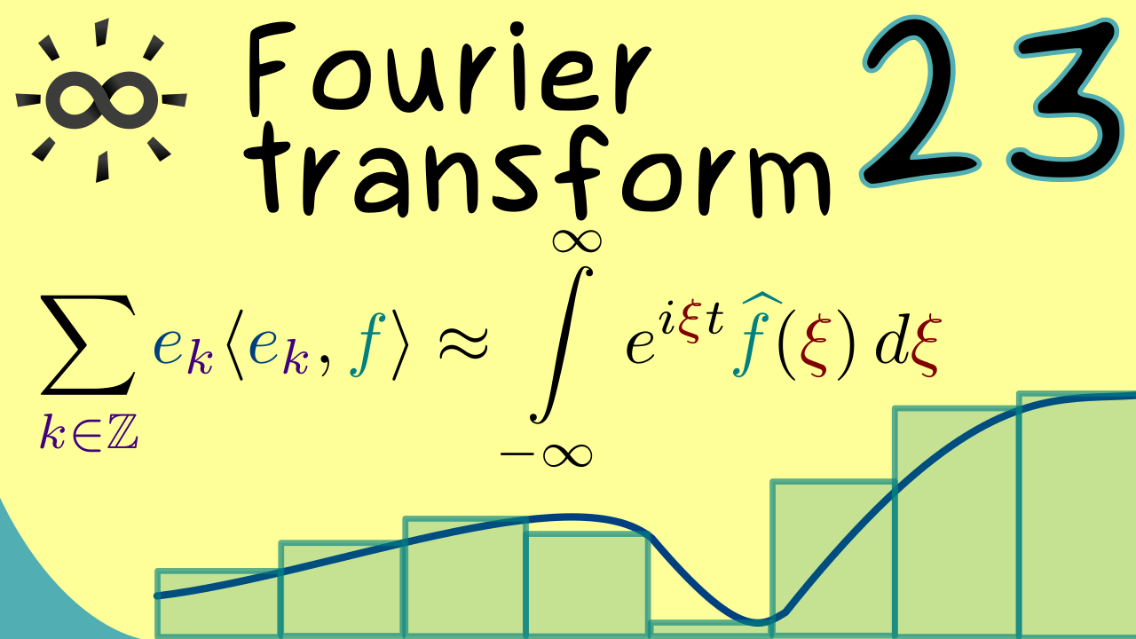
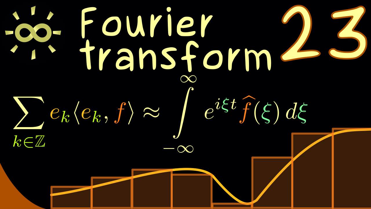
6 00:00:12.665 –> 00:00:15.485 we will finally build the bridge from the Fourier series
7 00:00:15.785 –> 00:00:18.125 to the continuous Fourier transform.
8 00:00:18.985 –> 00:00:21.835 This means that we can leave the periodic functions
9 00:00:21.835 –> 00:00:24.555 behind us and talk about the general concept
10 00:00:24.735 –> 00:00:26.235 of the Fourier transform.
11 00:00:26.825 –> 00:00:28.075 However, as always,
12 00:00:28.135 –> 00:00:30.635 before we discuss the details, I first want
13 00:00:30.635 –> 00:00:31.795 to thank all the nice people
14 00:00:31.895 –> 00:00:33.715 who support the channel on Steady, here on
15 00:00:33.715 –> 00:00:35.035 YouTube or via other means.
16 00:00:35.835 –> 00:00:38.955 Moreover, you should also know that you can download a lot
17 00:00:38.955 –> 00:00:41.995 of additional material with the link in the description.
18 00:00:42.905 –> 00:00:45.635 Okay, then let’s immediately start talking about the
19 00:00:45.635 –> 00:00:46.715 Fourier transform.
20 00:00:47.585 –> 00:00:49.445 In fact, the general definition works
21 00:00:49.545 –> 00:00:52.525 for integrable functions defined on Rn.
22 00:00:53.155 –> 00:00:56.125 Obviously, we can first consider the case n is equal
23 00:00:56.125 –> 00:00:57.205 to one such
24 00:00:57.205 –> 00:00:59.685 that we can see the connection to the Fourier series.
25 00:01:00.465 –> 00:01:02.245 And moreover, in general, the values
26 00:01:02.345 –> 00:01:04.365 of the function can be complex numbers
27 00:01:05.415 –> 00:01:08.635 and there the continuous Fourier transform can act
28 00:01:08.735 –> 00:01:10.315 as an integral transformation.
29 00:01:11.185 –> 00:01:15.085 And then what comes out is a function we call f hat defined
30 00:01:15.145 –> 00:01:16.605 on the frequency space.
31 00:01:17.375 –> 00:01:20.505 However, in contrast to the Fourier series approach,
32 00:01:21.125 –> 00:01:24.065 now the frequencies also form a continuum.
33 00:01:25.045 –> 00:01:28.465 So we are not in a countable set like the integer here.
34 00:01:28.525 –> 00:01:31.065 We also a function defined on Rn.
35 00:01:31.665 –> 00:01:34.155 Therefore to distinguish it to what we have done
36 00:01:34.435 –> 00:01:37.915 before, we can call it the continuous Fourier transform,
37 00:01:38.805 –> 00:01:41.505 but the overall idea still stays the same.
38 00:01:41.845 –> 00:01:43.985 We want to describe the original function
39 00:01:44.165 –> 00:01:46.505 by using cosine and sine functions.
40 00:01:47.165 –> 00:01:48.865 And the obvious difference here is
41 00:01:48.865 –> 00:01:50.665 that the original function does not have
42 00:01:50.665 –> 00:01:53.385 to be a two pi periodic function anymore.
43 00:01:54.065 –> 00:01:57.115 Therefore, I would say we first should write down the
44 00:01:57.115 –> 00:02:00.115 connection between the continuous Fourier transform
45 00:02:00.375 –> 00:02:02.235 and our original Fourier series.
46 00:02:03.025 –> 00:02:05.475 Therefore, we first stay one dimensional
47 00:02:05.855 –> 00:02:07.755 and periodic for our function f.
48 00:02:08.545 –> 00:02:12.755 This means we can sketch the graph of f on a compact domain.
49 00:02:13.695 –> 00:02:17.155 For example, we can say we have minus capital T here
50 00:02:17.455 –> 00:02:19.395 and plus capital T on the right,
51 00:02:20.345 –> 00:02:22.815 hence the function is two T periodic
52 00:02:23.035 –> 00:02:25.695 and it should be integrable on this domain.
53 00:02:26.835 –> 00:02:28.205 Therefore, the first idea
54 00:02:28.305 –> 00:02:31.725 to lose this periodicity requirement could be
55 00:02:31.725 –> 00:02:34.485 to increase this capital T more and more.
56 00:02:34.955 –> 00:02:37.685 However, it turns out that this doesn’t change anything
57 00:02:37.755 –> 00:02:40.685 because we can always scale the function down
58 00:02:40.785 –> 00:02:42.645 to two PI periodic functions.
59 00:02:43.545 –> 00:02:45.805 We just have to scale in the X direction
60 00:02:46.025 –> 00:02:48.125 by two pi over two T.
61 00:02:48.805 –> 00:02:51.305 In other words, we don’t lose any information
62 00:02:51.375 –> 00:02:55.225 because we just shrink the whole graph to a smaller domain.
63 00:02:55.895 –> 00:02:56.915 So the conclusion is
64 00:02:56.915 –> 00:03:00.085 that we can just use all our Fourier series methods
65 00:03:00.585 –> 00:03:02.365 to this new function on the bottom.
66 00:03:03.185 –> 00:03:05.525 So maybe we should give this function a new name.
67 00:03:05.775 –> 00:03:07.605 Let’s call it f tilde for the moment.
68 00:03:08.425 –> 00:03:11.085 And now let’s calculate the Fourier coefficients
69 00:03:11.265 –> 00:03:13.245 for this new function f tilde.
70 00:03:14.005 –> 00:03:16.505 And there you already know we just have the integral from
71 00:03:16.595 –> 00:03:20.985 minus pi to pi of the function e to the power minus
72 00:03:21.785 –> 00:03:25.405 i k x, and then we just multiply this
73 00:03:25.705 –> 00:03:27.165 by f tilde of x.
74 00:03:28.065 –> 00:03:30.965 So these are the Fourier coefficients of f tilde.
75 00:03:31.025 –> 00:03:32.485 But of course we want to go back
76 00:03:32.485 –> 00:03:35.965 to our original function f defined from the interval
77 00:03:36.045 –> 00:03:37.165 minus T to T.
78 00:03:37.845 –> 00:03:39.545 And this is not complicated at all.
79 00:03:39.845 –> 00:03:42.665 We just do a substitution in the integral
80 00:03:43.435 –> 00:03:46.375 and obviously the substitution is just the
81 00:03:46.375 –> 00:03:47.415 scaling from above.
82 00:03:48.245 –> 00:03:51.185 So our new variable can just be a lowercase t.
83 00:03:51.655 –> 00:03:55.745 Therefore our new integral here goes from minus capital T
84 00:03:56.045 –> 00:03:57.425 two plus capital T,
85 00:03:58.285 –> 00:04:00.545 and inside the interval instead of X,
86 00:04:00.645 –> 00:04:05.385 we write two pi over two times capital T times lowercase t.
87 00:04:06.175 –> 00:04:09.195 And there I can tell you that I will not cancel the two in
88 00:04:09.195 –> 00:04:12.715 the fraction because I want to emphasize the period we have
89 00:04:13.695 –> 00:04:16.195 on the lower level we are two PI periodic,
90 00:04:16.415 –> 00:04:19.755 and on the upper level we are two times T periodic.
91 00:04:20.555 –> 00:04:23.765 Okay? And now inside the integral we also have f tilde,
92 00:04:23.825 –> 00:04:26.845 scaled, which is our original function f.
93 00:04:27.465 –> 00:04:30.725 In other words, this here is simply f of t.
94 00:04:31.625 –> 00:04:34.885 And finally we have the last part of our substitution,
95 00:04:35.055 –> 00:04:37.085 which is the differential dt.
96 00:04:37.885 –> 00:04:40.385 And there you should see it cancels nicely
97 00:04:40.655 –> 00:04:42.785 with the factor in front of the integral.
98 00:04:43.375 –> 00:04:46.025 Therefore, our new factor in front is the new
99 00:04:46.025 –> 00:04:47.425 period, two times T.
100 00:04:48.135 –> 00:04:50.235 And moreover, we have our full result.
101 00:04:50.505 –> 00:04:52.515 This one is the final formula
102 00:04:52.895 –> 00:04:57.115 for the Fourier coefficient if the period is given by two T,
103 00:04:57.835 –> 00:05:01.055 in other words, these are the functions that form an ONS
104 00:05:01.075 –> 00:05:02.975 with our new period,
105 00:05:03.905 –> 00:05:07.015 which means if we consider square integrable functions,
106 00:05:07.275 –> 00:05:09.375 we can form the Fourier series
107 00:05:09.875 –> 00:05:12.935 and we know it converges, more precisely,
108 00:05:13.115 –> 00:05:16.215 we know it converges to the original function f
109 00:05:16.485 –> 00:05:18.095 with respect to the L2 norm.
110 00:05:19.095 –> 00:05:21.315 So we can write f as an infinite series
111 00:05:21.685 –> 00:05:23.995 where we have our new ONS involved
112 00:05:24.335 –> 00:05:26.755 and also the Fourier coefficients.
113 00:05:27.455 –> 00:05:29.755 And there, you know, the common notation we have
114 00:05:29.815 –> 00:05:32.195 for them is f head of k.
115 00:05:32.735 –> 00:05:34.635 So in the two pi periodic case,
116 00:05:34.735 –> 00:05:36.555 we know it’s given by this formula.
117 00:05:37.215 –> 00:05:39.635 And now by the substitution we have this
118 00:05:39.635 –> 00:05:41.155 formula for the general case.
119 00:05:41.915 –> 00:05:44.735 So in that sense, we don’t have anything new just instead
120 00:05:44.735 –> 00:05:47.255 of two pi, we talk about two T.
121 00:05:47.915 –> 00:05:51.925 However, this T is now changeable so we can make it larger
122 00:05:52.065 –> 00:05:53.165 and larger such
123 00:05:53.165 –> 00:05:55.885 that in a limit we cover the whole real number line
124 00:05:56.505 –> 00:05:58.245 and exactly this is our approach.
125 00:05:58.595 –> 00:06:01.245 What would happen in the limit T to infinity.
126 00:06:01.945 –> 00:06:04.805 We don’t have to be completely strict what we actually mean
127 00:06:04.825 –> 00:06:07.605 by the limit because it’s just a motivation here.
128 00:06:08.085 –> 00:06:10.095 Therefore, let’s first rewrite the formula
129 00:06:10.595 –> 00:06:12.495 and then apply some limit process.
130 00:06:13.645 –> 00:06:17.235 Again, here we go through all possible integer k,
131 00:06:17.535 –> 00:06:21.355 but the corresponding frequencies are not integer anymore.
132 00:06:22.515 –> 00:06:26.195 Actually the frequency we have is here between i and t.
133 00:06:26.775 –> 00:06:28.675 So let’s shorten it with a new notation.
134 00:06:28.845 –> 00:06:30.955 Let’s call it xi with index K.
135 00:06:31.785 –> 00:06:33.235 This is the Greek letter xi,
136 00:06:33.245 –> 00:06:35.835 which you can also pronounce as “ksai”.
137 00:06:36.735 –> 00:06:38.355 And indeed this definition helps us
138 00:06:38.425 –> 00:06:40.915 because now we can see the frequencies
139 00:06:41.375 –> 00:06:43.035 as points on the number line.
140 00:06:44.015 –> 00:06:47.475 For example, there we could have xi one, then the next one
141 00:06:47.475 –> 00:06:48.795 with index two and so on.
142 00:06:49.255 –> 00:06:51.915 And on the other hand we also have xi minus one,
143 00:06:52.195 –> 00:06:53.675 xi minus two, and so on.
144 00:06:54.295 –> 00:06:56.155 So we always have infinitely many.
145 00:06:56.455 –> 00:06:57.635 But now you should see
146 00:06:57.705 –> 00:07:00.635 what happens when we increase our capital T.
147 00:07:01.455 –> 00:07:04.665 Then because T is in the denominator of the definition,
148 00:07:05.085 –> 00:07:08.065 the points on the number line get closer together.
149 00:07:08.865 –> 00:07:10.565 So in this picture you already see
150 00:07:10.795 –> 00:07:13.685 that in some limit process T to infinity.
151 00:07:14.105 –> 00:07:17.245 In the end, we would cover all possible frequencies
152 00:07:17.385 –> 00:07:18.485 on the real number line.
153 00:07:19.295 –> 00:07:21.085 Again, it’s not completely precise,
154 00:07:21.305 –> 00:07:23.165 but it already makes sense for us.
155 00:07:23.945 –> 00:07:26.085 And indeed this will be our motivation
156 00:07:26.145 –> 00:07:27.605 for the next calculations.
157 00:07:28.465 –> 00:07:31.765 So first we use our xi_k here in the exponent
158 00:07:32.105 –> 00:07:34.365 and also the integral representation
159 00:07:34.585 –> 00:07:38.085 of the Fourier coefficient, which means also there
160 00:07:38.265 –> 00:07:42.045 inside the integral we have our xi_k for the frequency.
161 00:07:42.905 –> 00:07:46.125 And now actually our goal is to read this sum
162 00:07:46.345 –> 00:07:47.725 as a Riemann sum.
163 00:07:47.905 –> 00:07:50.045 So as an approximation for an integral,
164 00:07:50.575 –> 00:07:53.485 which means in the picture on the real number line here,
165 00:07:53.595 –> 00:07:56.805 what we actually need is the distance between two points.
166 00:07:57.625 –> 00:07:59.845 So something we could call delta xi
167 00:07:59.955 –> 00:08:02.925 because it’s the difference between two consecutive points.
168 00:08:03.775 –> 00:08:08.075 So more concretely we have xi of k minus xi
169 00:08:08.095 –> 00:08:09.195 of k minus one.
170 00:08:09.975 –> 00:08:12.875 And obviously this calculation is not complicated at all.
171 00:08:13.215 –> 00:08:17.435 We just get two pi over two T again, so quite simple,
172 00:08:17.615 –> 00:08:19.355 but this is the constant we have
173 00:08:19.355 –> 00:08:21.955 to introduce into our formula such
174 00:08:21.955 –> 00:08:23.395 that we can do the next steps.
175 00:08:24.255 –> 00:08:26.595 And in fact, it’s almost already there.
176 00:08:26.855 –> 00:08:30.435 We just have to introduce an additional factor one over two
177 00:08:30.495 –> 00:08:34.695 pi, which means we still have the whole integral divided
178 00:08:34.835 –> 00:08:38.615 by two pi and we can already see that as a function
179 00:08:38.805 –> 00:08:40.615 that depends on the real variable
180 00:08:41.135 –> 00:08:44.095 xi_k, and let’s already give it a good name.
181 00:08:44.465 –> 00:08:49.125 Let’s give it a thick hat and maybe also an index T
182 00:08:49.195 –> 00:08:51.325 because this one we want to increase
183 00:08:52.155 –> 00:08:55.605 and as already said, the variable name is a xi_k,
184 00:08:56.345 –> 00:08:57.765 and there you might already guess,
185 00:08:57.955 –> 00:09:00.885 this is almost already the Fourier transformation
186 00:09:00.905 –> 00:09:02.405 of f we want to get.
187 00:09:02.985 –> 00:09:04.405 But first for the motivation,
188 00:09:04.405 –> 00:09:05.965 you should read our sum like that.
189 00:09:06.265 –> 00:09:10.245 On the left we have the value of a function at a point xi_k,
190 00:09:10.785 –> 00:09:14.405 and then we multiply it with the distance on the x axis.
191 00:09:15.375 –> 00:09:18.185 This means if we have the graph of a function here,
192 00:09:18.605 –> 00:09:20.225 we sum up rectangles.
193 00:09:21.165 –> 00:09:23.265 In other words, what we have is an
194 00:09:23.265 –> 00:09:25.185 approximation of the integral.
195 00:09:25.955 –> 00:09:27.855 And moreover, we also already know
196 00:09:27.855 –> 00:09:30.415 that the partition here gets finer, finer.
197 00:09:30.675 –> 00:09:32.495 If we make T bigger and bigger
198 00:09:33.285 –> 00:09:34.665 or to keep it in a rough state,
199 00:09:34.885 –> 00:09:37.145 we could say if T is really large,
200 00:09:37.415 –> 00:09:39.945 then this whole infinite sum can be
201 00:09:40.345 –> 00:09:41.505 represented by an integral.
202 00:09:42.275 –> 00:09:45.095 For a really large T, it’s almost equal
203 00:09:45.155 –> 00:09:48.295 to the integral from minus infinity to plus infinity.
204 00:09:48.915 –> 00:09:53.135 And inside the integral, now we have the real variable xi,
205 00:09:53.805 –> 00:09:58.265 and as always, delta xi is now just d xi in the integral.
206 00:09:59.005 –> 00:10:01.725 Moreover, for f hat, we also want
207 00:10:01.725 –> 00:10:04.845 to integrate from minus infinity to plus infinity.
208 00:10:05.465 –> 00:10:08.805 But please never forget this factor one over two pi
209 00:10:09.145 –> 00:10:10.325 is always involved.
210 00:10:11.125 –> 00:10:14.825 We cannot get rid of it either it’s in the integral inside
211 00:10:15.085 –> 00:10:16.985 or on the outer integral here.
212 00:10:18.025 –> 00:10:20.475 Okay, so now please see this was the motivation.
213 00:10:20.545 –> 00:10:23.475 What should happen if we send T to infinity,
214 00:10:23.605 –> 00:10:27.635 which means we consider a non periodic function f defined on
215 00:10:27.635 –> 00:10:28.995 the whole real number line.
216 00:10:29.745 –> 00:10:33.755 Then the Fourier coefficients become this Fourier transform
217 00:10:33.925 –> 00:10:36.035 where xi can be any real number.
218 00:10:36.995 –> 00:10:39.775 And on the other hand the Fourier series goes
219 00:10:39.835 –> 00:10:41.175 to a whole integral
220 00:10:41.435 –> 00:10:44.335 and it should still represent the original function f.
221 00:10:45.215 –> 00:10:47.485 Hence for non periodic function f,
222 00:10:47.705 –> 00:10:50.445 we would define our Fourier transform like that.
223 00:10:51.025 –> 00:10:53.845 And then we get an inverse formula like this.
224 00:10:54.705 –> 00:10:58.685 And for this reason, the continuous Fourier transform has
225 00:10:58.835 –> 00:11:00.125 exactly this form.
226 00:11:00.685 –> 00:11:03.735 However, since the whole situation here is symmetric
227 00:11:03.965 –> 00:11:06.175 with two integrals on both sides,
228 00:11:06.605 –> 00:11:09.775 this factor one over two pi is a little bit annoying.
229 00:11:10.525 –> 00:11:14.335 Therefore one usually distributes this factor to both parts
230 00:11:14.755 –> 00:11:16.055 to keep this symmetry.
231 00:11:16.845 –> 00:11:19.695 Therefore, the definition of the Fourier transform
232 00:11:19.695 –> 00:11:24.375 of f can be written with a factor one over this square root
233 00:11:24.595 –> 00:11:26.375 of two pi in front of it.
234 00:11:27.105 –> 00:11:28.515 Otherwise nothing changes.
235 00:11:28.975 –> 00:11:31.755 Inside the integral we have the exponential function,
236 00:11:31.935 –> 00:11:33.115 but with a minus sign.
237 00:11:33.665 –> 00:11:37.115 Otherwise we just have our function f inside the integral.
238 00:11:37.335 –> 00:11:38.835 So the only requirement
239 00:11:38.835 –> 00:11:41.515 for the continuous Fourier transform is
240 00:11:41.515 –> 00:11:43.675 that we have an integrable function,
241 00:11:44.465 –> 00:11:48.525 or in short, you would write f is chosen from L one.
242 00:11:49.115 –> 00:11:51.325 However, there it’s not clear at all
243 00:11:51.435 –> 00:11:54.165 that our f hat is in L one as well.
244 00:11:55.045 –> 00:11:57.635 Hence this inverse formula might not be
245 00:11:57.695 –> 00:11:59.235 so general as we want it.
246 00:11:59.975 –> 00:12:01.555 But of course this is what we have
247 00:12:01.555 –> 00:12:04.155 to discuss in all details in future videos.
248 00:12:05.015 –> 00:12:06.795 And there I can already tell you this.
249 00:12:06.795 –> 00:12:10.195 Step to Rn in this definition here is not a problem at all.
250 00:12:11.015 –> 00:12:14.275 So this is something we can already do in the next video.
251 00:12:15.075 –> 00:12:16.295 So I really hope I meet you today
252 00:12:16.295 –> 00:12:17.655 again, and have a nice day.
253 00:12:17.965 –> 00:12:18.455 Bye-bye.
-
Quiz Content (n/a)
-
Date of video: 2025-05-12
-
Last update: 2025-09