
-
Title: Riemann–Lebesgue Lemma for Fourier Series
-
Series: Fourier Transform
-
Chapter: Fourier Series
-
YouTube-Title: Fourier Transform 22 | Riemann–Lebesgue Lemma for Fourier Series
-
Bright video: Watch on YouTube
-
Dark video: Watch on YouTube
-
Ad-free video: Watch Vimeo video
-
Forum: Ask a question in Mattermost
-
Dark-PDF: Download PDF version of the dark video
-
Print-PDF: Download printable PDF version
-
Thumbnail (bright): Download PNG
-
Thumbnail (dark): Download PNG
-
Subtitle on GitHub: ft22_sub_eng.srt
-
Download bright video: Link on Vimeo
-
Download dark video: Link on Vimeo
-
Related videos:
-
Timestamps (n/a)
-
Subtitle in English
1 00:00:00.685 –> 00:00:02.035 Hello and welcome back
2 00:00:02.055 –> 00:00:04.475 to Fourier Transform the video series
3 00:00:04.475 –> 00:00:07.515 where we talk a lot about so-called Fourier series.
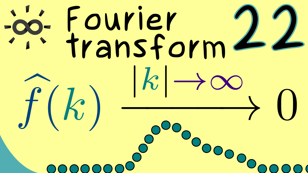
4 00:00:08.455 –> 00:00:11.835 And indeed in today’s part 22, we will tackle the famous
5 00:00:12.435 –> 00:00:13.515 Riemann-Lebesgue lemma.
6 00:00:13.915 –> 00:00:15.965 Roughly speaking, this one tell us
7 00:00:16.075 –> 00:00:19.725 that the Fourier coefficients form a sequence which is
8 00:00:20.165 –> 00:00:21.565 convergent with limit zero.
9 00:00:22.255 –> 00:00:25.465 However, before we formulate this theorem, I first want
10 00:00:25.465 –> 00:00:26.865 to thank all the nice people
11 00:00:26.925 –> 00:00:28.905 who support this channel on Steady, here on
12 00:00:28.905 –> 00:00:30.425 YouTube, or via other means.
13 00:00:31.125 –> 00:00:34.105 And as a reminder, a Steady membership gives you access
14 00:00:34.105 –> 00:00:36.945 to a lot of additional material like PDF versions,
15 00:00:36.995 –> 00:00:38.945 early access and quizzes.
16 00:00:39.935 –> 00:00:41.835 So please use the link in the description
17 00:00:41.895 –> 00:00:43.595 to download the additional material.
18 00:00:44.455 –> 00:00:46.155 So let’s start by recalling
19 00:00:46.155 –> 00:00:49.475 that we have defined the Fourier series in L one.
20 00:00:50.185 –> 00:00:51.515 This was not a problem at all
21 00:00:51.515 –> 00:00:55.755 because the Fourier coefficients given by this integral exist
22 00:00:55.855 –> 00:00:58.075 for any L one function f.
23 00:00:58.895 –> 00:01:01.675 And moreover, we also have introduced a new name
24 00:01:01.735 –> 00:01:05.555 for the Fourier coefficients, namely we call them f head
25 00:01:05.575 –> 00:01:09.985 of k, which immediately implies that we get a whole sequence
26 00:01:10.085 –> 00:01:11.385 of complex numbers here.
27 00:01:12.125 –> 00:01:14.425 And now a natural question we could ask is
28 00:01:14.775 –> 00:01:18.065 what can we say about this sequence of complex numbers?
29 00:01:18.885 –> 00:01:20.545 And one famous answer for
30 00:01:20.545 –> 00:01:23.985 that question is the so-called Riemann-Lebesgue Lemma.
31 00:01:24.605 –> 00:01:27.385 For historical reasons, it’s still called a lemma,
32 00:01:27.565 –> 00:01:30.625 but nevertheless, it’s a really important result in the
33 00:01:30.625 –> 00:01:31.905 theory of Fourier series.
34 00:01:32.725 –> 00:01:36.665 And it helps us that for any L one function, the sequence
35 00:01:36.665 –> 00:01:40.465 of Fourier coefficients is a convergent sequence for k
36 00:01:40.525 –> 00:01:42.105 to plus or minus infinity.
37 00:01:42.865 –> 00:01:45.755 More precisely we can write that this limit exists
38 00:01:46.215 –> 00:01:49.875 and is equal to zero, so eventually measured
39 00:01:49.875 –> 00:01:50.875 with the absolute value,
40 00:01:51.175 –> 00:01:53.675 the sequence becomes smaller and smaller.
41 00:01:54.375 –> 00:01:56.875 So we cannot say how fast it goes to zero,
42 00:01:57.015 –> 00:01:59.035 but at least we know it goes to zero.
43 00:01:59.815 –> 00:02:02.825 This means the linear map we have denoted by a hat
44 00:02:03.615 –> 00:02:06.425 goes from L one into the space
45 00:02:06.485 –> 00:02:08.985 of convergence sequences with limit zero.
46 00:02:09.845 –> 00:02:13.625 And the common notation for this space is simply c
47 00:02:13.695 –> 00:02:14.825 with index zero.
48 00:02:15.645 –> 00:02:17.065 So not a complicated space.
49 00:02:17.205 –> 00:02:19.545 And now we know by the Riemann-Lebesgue lemma
50 00:02:19.855 –> 00:02:23.505 that all the sequences given by Fourier coefficients lie
51 00:02:23.605 –> 00:02:24.625 inside that space.
52 00:02:25.175 –> 00:02:28.825 However, what we definitely don’t know is if this map here
53 00:02:28.845 –> 00:02:30.225 is also surjective.
54 00:02:31.045 –> 00:02:32.785 And at this point I can already tell you
55 00:02:32.785 –> 00:02:34.065 that we don’t have that.
56 00:02:34.405 –> 00:02:38.105 So this hat map will not hit all the sequences tending
57 00:02:38.105 –> 00:02:39.585 to zero on the right hand side.
58 00:02:40.355 –> 00:02:42.985 Hence, not every sequence here is given
59 00:02:43.125 –> 00:02:45.625 by the Fourier coefficients of an L one function.
60 00:02:46.235 –> 00:02:48.045 However, this is not a topic for today
61 00:02:48.075 –> 00:02:50.405 because today we will just prove
62 00:02:50.435 –> 00:02:53.405 that the hat map maps into the sequence space.
63 00:02:54.195 –> 00:02:56.335 For the proof of that, you should first note
64 00:02:56.445 –> 00:02:58.895 that we already know it for L two functions.
65 00:02:59.845 –> 00:03:01.975 This is quite clear because for the space
66 00:03:01.995 –> 00:03:05.535 of square integrable functions, we have Parseval’s identity.
67 00:03:06.395 –> 00:03:09.135 And this one tells us that the corresponding sequence
68 00:03:09.235 –> 00:03:12.175 of Fourier coefficients is square summable.
69 00:03:12.845 –> 00:03:14.505 And by using the mathematical language,
70 00:03:14.505 –> 00:03:17.225 we would just write this sequence is an element
71 00:03:17.605 –> 00:03:18.865 of small l two.
72 00:03:19.595 –> 00:03:23.455 And obviously tending to zero at infinity is necessary
73 00:03:23.635 –> 00:03:26.095 for a sequence being square summable,
74 00:03:26.675 –> 00:03:30.495 or in other words, l two is a proper subset of c zero.
75 00:03:31.235 –> 00:03:33.215 In other words, this result is not new
76 00:03:33.215 –> 00:03:36.615 for us at all if we just consider L two functions.
77 00:03:37.215 –> 00:03:40.625 However, if we take a function which is in L one,
78 00:03:40.885 –> 00:03:43.705 but not in L two, we don’t know anything yet.
79 00:03:44.385 –> 00:03:45.925 So for example, the graph
80 00:03:45.945 –> 00:03:48.765 of such a problematic function could look like this.
81 00:03:49.715 –> 00:03:51.815 It could explode somewhere, so it doesn’t have
82 00:03:51.815 –> 00:03:52.815 to be bounded at all.
83 00:03:53.845 –> 00:03:56.945 The only requirement we need is that the integral
84 00:03:56.965 –> 00:03:59.665 of the absolute value is still a finite number.
85 00:04:00.395 –> 00:04:03.105 Hence in this picture we would say that this area
86 00:04:03.215 –> 00:04:06.425 that stretches to infinity still has a finite value,
87 00:04:07.165 –> 00:04:08.385 but we cannot assume
88 00:04:08.385 –> 00:04:11.425 that the same thing holds when we have the absolute value
89 00:04:11.445 –> 00:04:14.035 of f squared there.
90 00:04:14.135 –> 00:04:15.995 It could definitely happen that the value
91 00:04:16.175 –> 00:04:17.915 of the area is infinity,
92 00:04:18.455 –> 00:04:21.355 and this is exactly the case we need to address now.
93 00:04:22.055 –> 00:04:26.155 And there the simple idea is to make the function square integrable
94 00:04:26.295 –> 00:04:27.515 by making it bounded.
95 00:04:28.135 –> 00:04:31.035 In other words, we just cut the function at the top.
96 00:04:31.935 –> 00:04:34.835 And of course this nice picture is correct for any function.
97 00:04:35.025 –> 00:04:38.315 When we say the craft is of the absolute value of f,
98 00:04:39.065 –> 00:04:40.875 then everything here is non-negative
99 00:04:41.135 –> 00:04:42.875 and we just have to cut at the top.
100 00:04:43.465 –> 00:04:45.915 However, this new cut function should still be
101 00:04:45.995 –> 00:04:47.075 a complex value to one.
102 00:04:47.255 –> 00:04:51.455 So let’s call it fN. It’s a two pi periodic function.
103 00:04:51.635 –> 00:04:54.135 So we can define it on the whole real number line.
104 00:04:54.715 –> 00:04:57.295 And actually the definition is already given in the picture,
105 00:04:57.715 –> 00:04:59.335 we just distinguish two cases.
106 00:05:00.475 –> 00:05:01.535 If the absolute value
107 00:05:01.675 –> 00:05:05.655 of f at a given point x is less than our given N,
108 00:05:06.525 –> 00:05:08.255 then we don’t want to do anything.
109 00:05:08.635 –> 00:05:11.535 We should still have the same value f of x.
110 00:05:12.305 –> 00:05:13.845 On the other hand, in the case
111 00:05:13.845 –> 00:05:16.645 that we are larger than this given N, then we want
112 00:05:16.645 –> 00:05:17.645 to cut the function.
113 00:05:18.415 –> 00:05:20.635 And then to make it simple, we just set it
114 00:05:20.635 –> 00:05:22.035 to the given value N.
115 00:05:22.775 –> 00:05:24.515 And obviously this definition works
116 00:05:24.575 –> 00:05:27.675 for any fixed natural number, capital N.
117 00:05:28.295 –> 00:05:30.875 And now the good thing is with this bounded fN,
118 00:05:30.935 –> 00:05:34.075 we are back in our best case, we are in L two.
119 00:05:34.825 –> 00:05:37.125 So for this cut version of the function,
120 00:05:37.265 –> 00:05:39.445 we can use Parseval’s identity again,
121 00:05:40.275 –> 00:05:41.655 indeed, this is the whole idea.
122 00:05:41.875 –> 00:05:44.095 And then we just have to build the bridge back
123 00:05:44.095 –> 00:05:45.735 to our original function f.
124 00:05:46.635 –> 00:05:49.615 And for that we can use a nice convergence result,
125 00:05:49.825 –> 00:05:53.575 which is known as Lebesgue’s dominated convergence theorem.
126 00:05:54.445 –> 00:05:56.375 This is a theorem about integration
127 00:05:56.675 –> 00:05:59.805 and I have discussed it in my measure theory series.
128 00:06:00.625 –> 00:06:02.085 So if you’re interested in the proof,
129 00:06:02.185 –> 00:06:03.245 you can check it out there.
130 00:06:03.425 –> 00:06:05.245 But here we just want to apply it.
131 00:06:05.735 –> 00:06:08.185 Therefore, I first tell you the assumptions we need
132 00:06:08.445 –> 00:06:11.715 and then the implication, as the name suggests,
133 00:06:11.715 –> 00:06:13.075 we need a dominating function,
134 00:06:13.255 –> 00:06:15.875 and this one can be our original function.
135 00:06:16.075 –> 00:06:18.975 f indeed this inequality is quite clear
136 00:06:19.005 –> 00:06:20.135 because this is
137 00:06:20.135 –> 00:06:22.935 how we have defined the cut version of the function.
138 00:06:23.735 –> 00:06:27.595 And to be precise, we need this inequality for every N in N
139 00:06:27.855 –> 00:06:30.515 and for every x in R, almost everywhere,
140 00:06:31.245 –> 00:06:32.505 almost everywhere makes sense
141 00:06:32.505 –> 00:06:35.545 because we only talk about the equivalence classes
142 00:06:35.685 –> 00:06:37.105 of function here anyway.
143 00:06:37.865 –> 00:06:39.765 And on the other hand, we also want
144 00:06:39.765 –> 00:06:41.485 to have pointwise convergence
145 00:06:41.785 –> 00:06:43.365 for this sequence of functions.
146 00:06:44.195 –> 00:06:46.605 This means when N tends to infinity,
147 00:06:47.035 –> 00:06:49.005 then this should tend to f of x.
148 00:06:49.995 –> 00:06:52.405 Also, this assumption should hold almost everywhere
149 00:06:52.745 –> 00:06:55.405 and it’s not hard to see that we have that indeed.
150 00:06:56.105 –> 00:06:58.285 If we increase N, then we cut less
151 00:06:58.345 –> 00:07:00.165 and less of the original function,
152 00:07:00.815 –> 00:07:03.065 therefore for a fixed point x here,
153 00:07:03.275 –> 00:07:05.505 eventually this convergence will happen.
154 00:07:06.245 –> 00:07:09.665 And now LabX dominated convergence theorem says if you have
155 00:07:09.755 –> 00:07:13.665 these two assumptions, then we also have convergence
156 00:07:13.685 –> 00:07:17.385 of the sequence to f with respect to the L one norm
157 00:07:18.085 –> 00:07:21.585 or to say it in other words, we also have the convergence
158 00:07:21.885 –> 00:07:22.945 of the integral.
159 00:07:23.965 –> 00:07:26.465 So inside the integral we have the difference
160 00:07:26.465 –> 00:07:28.025 between fN and f.
161 00:07:28.885 –> 00:07:32.105 And even after integrating, that still goes
162 00:07:32.165 –> 00:07:34.745 to zero when N tends to infinity.
163 00:07:35.455 –> 00:07:37.235 And exactly this is the result
164 00:07:37.255 –> 00:07:39.955 of Lebesgue’s dominated convergence theorem.
165 00:07:40.655 –> 00:07:42.515 It just gives us the justification
166 00:07:42.815 –> 00:07:44.995 to push the limit into the integration.
167 00:07:45.795 –> 00:07:49.135 And of course the question for us is now can we use it
168 00:07:49.195 –> 00:07:50.895 for the Fourier coefficients?
169 00:07:51.645 –> 00:07:54.945 The basic idea would be to use the Fourier coefficients
170 00:07:55.085 –> 00:07:57.345 of our L two function fN,
171 00:07:58.205 –> 00:08:00.585 and then by increasing the natural number N,
172 00:08:00.805 –> 00:08:03.265 we should approximate our Fourier coefficient
173 00:08:03.265 –> 00:08:04.745 of f better and better.
174 00:08:05.565 –> 00:08:06.625 So how can we see that?
175 00:08:06.715 –> 00:08:10.545 Maybe first we use the definition of the Fourier coefficient.
176 00:08:11.085 –> 00:08:12.585 So here we would have the difference
177 00:08:12.585 –> 00:08:14.145 between two integrations,
178 00:08:14.445 –> 00:08:18.025 but we can also put it together, which means we have fN
179 00:08:18.025 –> 00:08:21.705 of X minus f of X times the exponential function.
180 00:08:22.445 –> 00:08:24.745 And now since we only care about the difference
181 00:08:24.745 –> 00:08:26.545 of the two complex numbers on the left,
182 00:08:27.045 –> 00:08:30.225 we can also consider the absolute value on both sides.
183 00:08:31.165 –> 00:08:34.105 And by having that, we can use the triangle inequality
184 00:08:34.645 –> 00:08:37.265 for the integration, which simply means
185 00:08:37.265 –> 00:08:40.825 that we can push the absolute value into the integration.
186 00:08:41.565 –> 00:08:43.585 And there please recall the modulus
187 00:08:43.605 –> 00:08:45.505 of the complex exponential function.
188 00:08:45.505 –> 00:08:47.505 This form is equal to one.
189 00:08:48.095 –> 00:08:51.035 So the only thing that remains inside is the distance
190 00:08:51.035 –> 00:08:53.395 between fN of X and f of X.
191 00:08:54.095 –> 00:08:56.725 And there we already know that we can make this as small
192 00:08:56.725 –> 00:08:59.085 as we want just by increasing N.
193 00:08:59.845 –> 00:09:01.765 Moreover, we also recognize
194 00:09:01.835 –> 00:09:04.285 that this does not depend on the chosen
195 00:09:04.605 –> 00:09:05.645 K on the left hand side.
196 00:09:06.335 –> 00:09:09.435 So the conclusion is that all the Fourier coefficients
197 00:09:09.535 –> 00:09:14.195 of f can be approximated by the Fourier coefficients of fN.
198 00:09:15.005 –> 00:09:16.665 And with that, we almost have it.
199 00:09:16.725 –> 00:09:20.225 We just have to put everything together to be clear.
200 00:09:20.485 –> 00:09:22.185 Now we have two different kinds
201 00:09:22.185 –> 00:09:24.265 of convergence we can combine.
202 00:09:24.875 –> 00:09:27.025 Maybe let’s first write down the second one
203 00:09:27.055 –> 00:09:29.025 because we just have discussed it.
204 00:09:29.645 –> 00:09:33.875 It means for any given epsilon we find an index capital N,
205 00:09:34.065 –> 00:09:37.275 such that the right hand side here is smaller than epsilon,
206 00:09:37.685 –> 00:09:38.835 which also implies
207 00:09:38.835 –> 00:09:41.595 that the left hand side is smaller than epsilon
208 00:09:41.815 –> 00:09:43.115 for any given K.
209 00:09:43.915 –> 00:09:46.135 And now if you want, we can also make it
210 00:09:46.165 –> 00:09:47.455 less than epsilon half.
211 00:09:48.525 –> 00:09:49.735 Okay, so this should be clear
212 00:09:49.735 –> 00:09:52.055 because it’s exactly what came out
213 00:09:52.055 –> 00:09:54.415 of Lebesgue’s dominated convergence theorum.
214 00:09:55.155 –> 00:09:56.495 And now on the other hand,
215 00:09:56.675 –> 00:09:59.255 the first convergence we have already discussed at the
216 00:09:59.255 –> 00:10:01.575 beginning of the proof, it’s just
217 00:10:01.575 –> 00:10:04.255 that every fN function lies in L two.
218 00:10:04.475 –> 00:10:09.215 So they’re all satisfy Parseval’s identity, which implies
219 00:10:09.215 –> 00:10:14.095 that after an index capital K, all the sequence members lie
220 00:10:14.275 –> 00:10:15.535 inside an epsilon ball.
221 00:10:16.305 –> 00:10:18.165 And this is true in both directions.
222 00:10:18.305 –> 00:10:21.285 So it holds for plus infinity and minus infinity.
223 00:10:22.165 –> 00:10:24.315 Hence, we can just write that the absolute value
224 00:10:24.335 –> 00:10:27.595 of k is greater or equal than the given capital K.
225 00:10:28.455 –> 00:10:31.835 And now being inside the epsilon ball means that the modelus
226 00:10:31.935 –> 00:10:34.795 of the complex number is less than epsilon.
227 00:10:35.645 –> 00:10:38.225 And also here we can choose the radius of the ball
228 00:10:38.365 –> 00:10:41.245 as epsilon half as well, very well
229 00:10:41.475 –> 00:10:43.245 Both statements here are correct
230 00:10:43.545 –> 00:10:46.125 and we can combine them to get our result,
231 00:10:46.655 –> 00:10:49.845 which means if you give me an epsilon greater than zero,
232 00:10:50.325 –> 00:10:54.405 I can choose a capital N and a capital K more precisely
233 00:10:54.495 –> 00:10:56.685 First, we choose the capital N according
234 00:10:56.705 –> 00:10:57.925 to the second statement.
235 00:10:58.305 –> 00:11:00.165 And then according to epsilon
236 00:11:00.265 –> 00:11:02.365 and N, we can choose the capital K
237 00:11:02.365 –> 00:11:03.765 according to the first statement.
238 00:11:04.465 –> 00:11:07.455 Afterwards, we can combine both statements again
239 00:11:07.715 –> 00:11:10.415 and get something out for integer k.
240 00:11:11.075 –> 00:11:13.975 But of course the first statement gives us the requirement
241 00:11:14.125 –> 00:11:16.295 that the absolute value of k is greater
242 00:11:16.295 –> 00:11:17.695 or equal than capital K.
243 00:11:18.355 –> 00:11:21.415 And now for all these integer k, we want to show
244 00:11:21.415 –> 00:11:24.375 that the absolute value of the Fourier coefficient
245 00:11:24.435 –> 00:11:27.295 of f is less than our given epsilon
246 00:11:27.775 –> 00:11:32.465 because exactly this would be the convergence to zero for k
247 00:11:32.465 –> 00:11:33.945 to plus or minus infinity.
248 00:11:34.645 –> 00:11:36.305 And with that, we almost have it.
249 00:11:36.325 –> 00:11:40.065 We just have to introduce our fN into the equation again.
250 00:11:40.685 –> 00:11:44.665 So we subtract and add the Fourier coefficient, fN hat,
251 00:11:45.465 –> 00:11:48.485 and then we can simply use the triangle inequality.
252 00:11:49.365 –> 00:11:50.745 And then you might already see it.
253 00:11:50.885 –> 00:11:54.205 We have exactly the two parts where we have an estimate
254 00:11:54.865 –> 00:11:58.085 and that’s the whole reason why we chose epsilon half before.
255 00:11:58.875 –> 00:12:00.335 So the modulus of this Fourier
256 00:12:00.455 –> 00:12:02.535 coefficient here is less than epsilon,
257 00:12:02.835 –> 00:12:05.695 and this holds for infinitely many indices
258 00:12:05.945 –> 00:12:07.295 after a starting index.
259 00:12:08.255 –> 00:12:11.155 In other words, we can make it arbitrarily small eventually.
260 00:12:11.415 –> 00:12:14.435 And this is exactly the convergence we wanted to show.
261 00:12:15.015 –> 00:12:17.875 And with that, the Riemann-Lebesgue lemma is proven.
262 00:12:18.755 –> 00:12:20.535 Please note here we have shown it
263 00:12:20.535 –> 00:12:22.495 for the complex Fourier coefficients,
264 00:12:22.635 –> 00:12:25.255 but of course it also holds for the real ones.
265 00:12:26.025 –> 00:12:29.275 This just follows from the standard relation between the two
266 00:12:29.875 –> 00:12:31.555 representations of the Fourier series.
267 00:12:32.265 –> 00:12:35.715 Therefore, the Riemann-Lebesgue lemma might also help you if
268 00:12:35.715 –> 00:12:37.835 you have an integral with a cosine
269 00:12:37.835 –> 00:12:39.075 or sine function involved.
270 00:12:39.955 –> 00:12:41.685 Okay, with that, I close this video
271 00:12:41.905 –> 00:12:43.845 and I really hope I meet you next time.
272 00:12:44.075 –> 00:12:44.565 Bye-bye.
-
Quiz Content (n/a)
-
Date of video: 2025-05-07
-
Last update: 2025-09